Mathematical modelling of a biofilm: The Adomian decomposition method ()
1. INTRODUCTION
Microorganisms biofilms adhere to the interfaces between gas and liquid phases, liquid and solid phases, or two liquid phases [1]. Their activity can have an adverse effect, e.g., biofilms damage materials [2], and water purification technology [3]. The situation is largely similar to the case of heterogeneous reaction in a porous layer [4,5]; however, for the biofilm kinetics, there are a number of specific features. The dependence of the biochemical reaction rate on a substrate concentration is described by a saturating curve and can not be characterized by a power function [3,6]. Dueck et al. [7-9] described the mathematical modeling of evaluation of biofilm with allowance for its erosion. Recently, Min kov et al. [10] obtained the analytical expression for the substrate flux in to the biofilm as the function of volumetric flow rate of the substrate solution. To my knowledge no rigorous analytical solution of concentration of substrate and flux into the biofilm for a square law of microbial death rate with steady-state conditions has been reported. The purpose of this communication is to derive approximate analytical expressions for the steady-state concentration of substrate and flux into the biofilm using the Adomian decomposition method for all values of biofilm thickness and substrate concentration outside the biofilm.
2. MATHEMATICAL FORMULATION OF THE PROBLEM
It is assumed that the substrate consumption is described by the Michaelis-Menten kinetics. The Equation of which are derived on the basis of the theory of enzymatic reactions [3,5] on the particle surface of biofilm [10] is of the following form:
 (1)
(1)
The boundary conditions are
 (2)
(2)
 (3)
(3)
The biomass balance [10].
 (4)
(4)
From Eq.4, the concentration of active biomass can be expressed through the substrate concentration. Now the Eq.1 can be written in the form
 (5)
(5)
where Sf is the substrate concentration in the biofilm, K is the Michaelis-Menten constant, z is the co-ordinate, Lf is the biofilm thickness, Df is the diffusion coefficient within the biofilm, b is the Microbial death constant, q is the substrate consumption rate constant, S1 is the substrate concentration outside the bioflim and Y is the biomass yield per unit amount of substrate consumed respectively. The non-linear ODE (Eq.5) is made dimensionless by defining the following parameters:
 (6)
(6)
The above Eq.5 reduces to the following dimensionless form:
 (7)
(7)
 (8)
(8)
 (9)
(9)
The dimensionless concentration flux into the biofilm is given by
 (10)
(10)
3. SOLUTION OF BOUNDARY VALUE PROBLEM BY THE ADOMIAN DECOMPOSITION METHOD
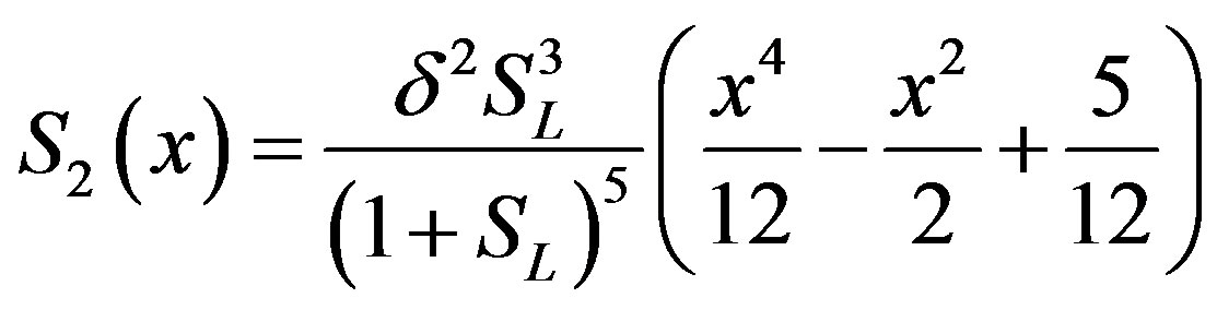
The Adomian’s decomposition method has been successfully applied to linear and nonlinear problems. One of its advantages is that it provides a rapid convergent series solution. However, in this method, some modifications are proposed by several authors [11-15]. By applying the Adomian’s decomposition method, a new iterative method to compute nonlinear Equations are developed. The Adomian decomposition method is an extremely simple method [11-15] to solve the non-linear differential Equations. First iteration is enough. Furthermore, the obtained result is of high accuracy. Using this Adomian decomposition method (see Appendix A and B), the solution of Eq.7 becomes:
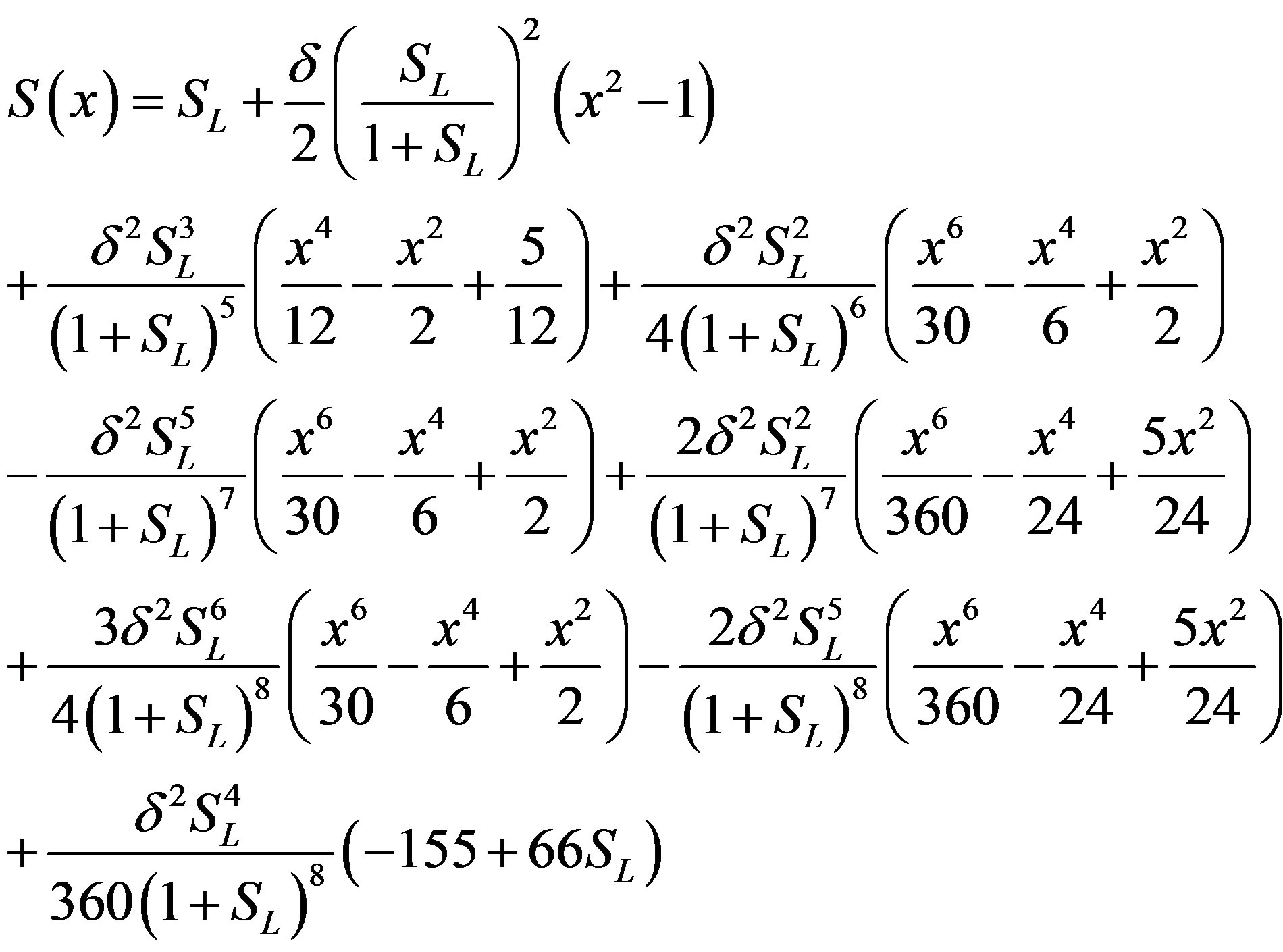 (11)
(11)
The solution of concentration flux into the biofilm is obtained as
 (12)
(12)
4. NUMERICAL SIMULATION
The non-linear differentials Eq.7 is also solved by numerical methods. The function bvp4c in Matlab software which is a function of solving two-point boundary value problems (BVPs) for ordinary differential equations is used to solve this equation. The Matlab program is also given in Appendix C. Its numerical solution is compared with Adomian decomposition method in Tables 1 and 2 and Figures 1-3 for various value of parameters.
5. RESULTS AND DISCUSSION
An approximate analytical expression of concentrations S is given in the Eq.11. The concentration  is plotted in Figures 1-3 for various values of δ and
 . From these figures, it is evident that the value of concentration gradually increases as the dimensionless biofilm thickness δ decreases. Figures 4 to 5 represent the concentration
  for various values of SL. From these this figures it is observed that, the value of the concentration increases when SL increases. When
 , the
, the
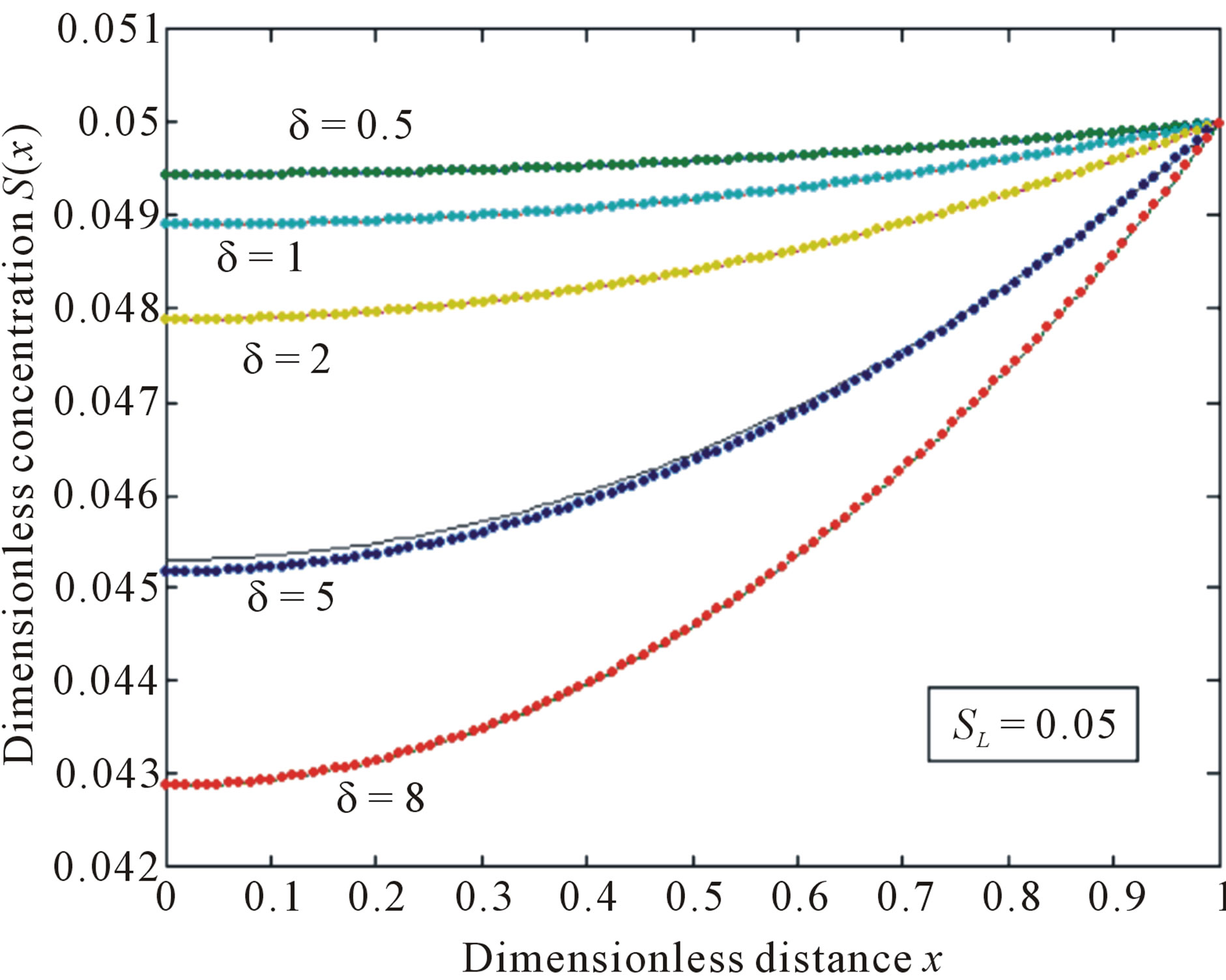
Figure 1. Normalized concentration profile S(x) as a function of dimensionless distance x. The concentrations were computed using Eq.11 for various values of the δ when SL = 0.05, (—) denotes Eq.11 and (…) denotes the numerical simulation.
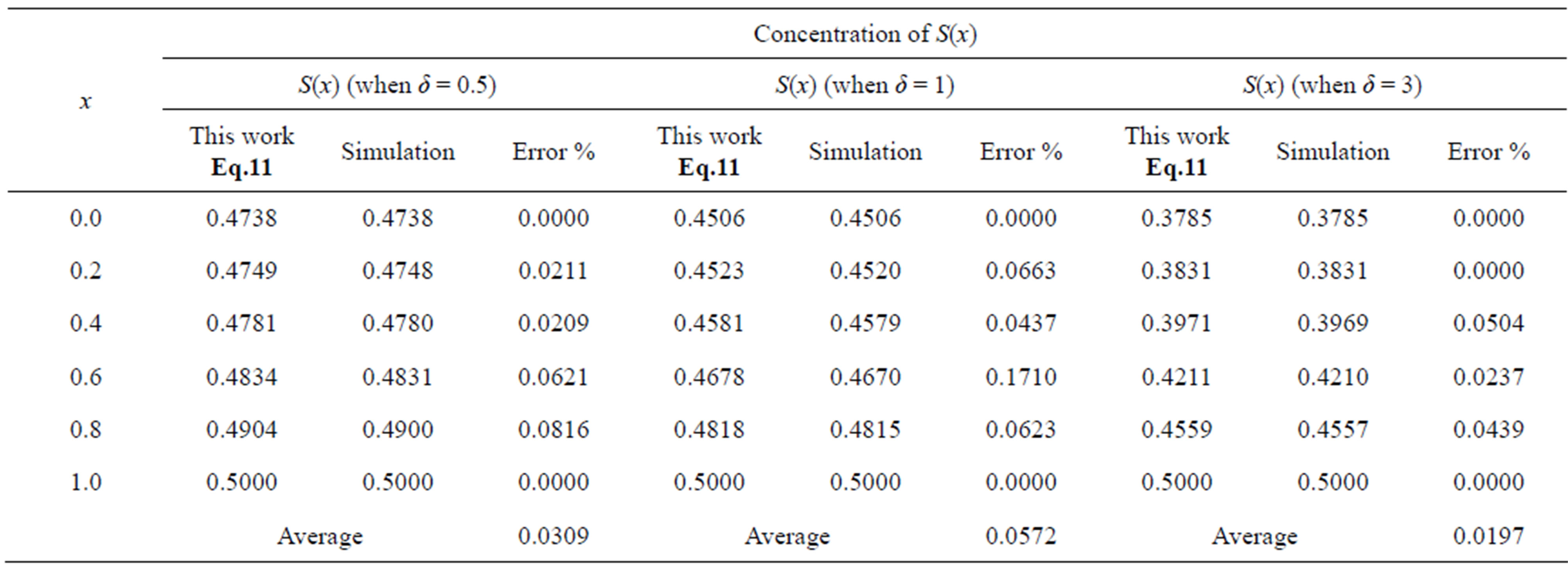
Table 1. Comparison of normalized steady-state concentration S(x) with simulation results for various values of x and for some fixed values of SL = 0.5.
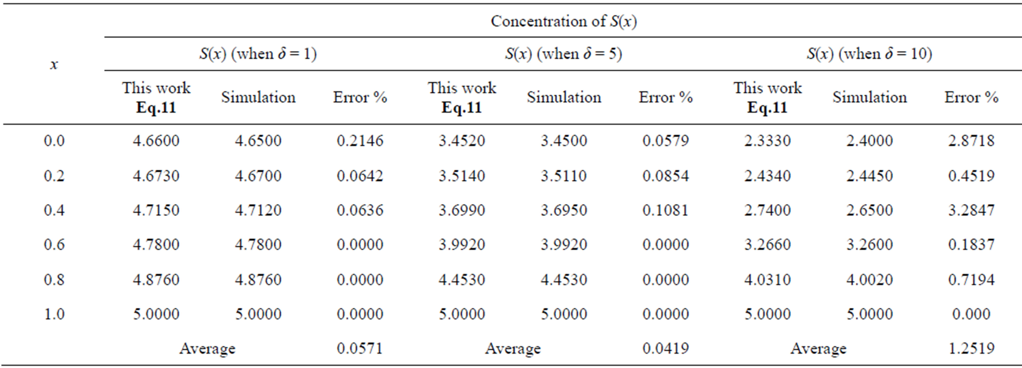
Table 2. Comparison of normalized steady-state concentration S(x) with simulation results for various values of x and for some fixed values of SL = 5.
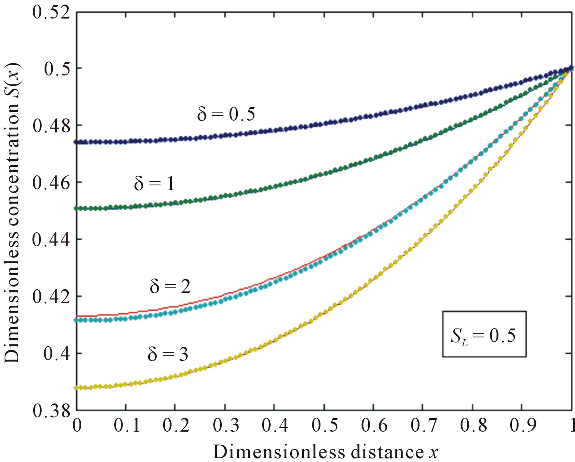
Figure 2. Normalized concentration profile S(x) as a function of dimensionless distance x. The concentrations were computed using Eq.11 for various values of the δ when SL = 0.5, (—) denotes Eq.11 and (…) denotes the numerical simulation.

Figure 3. Normalized concentration profile S(x) as a function of dimensionless distance x. The concentrations were computed using Eq.11 for various values of the δ when SL = 5, (—) denotes Eq.11 and (…) denotes the numerical simulation.

Figure 4. Normalized concentration profile S(x) as a function of dimensionless distance x. The concentrations were computed using Eq.11 for various values of the SL when δ = 10, (—) denotes Eq.11 and (…) denotes the numerical simulation.
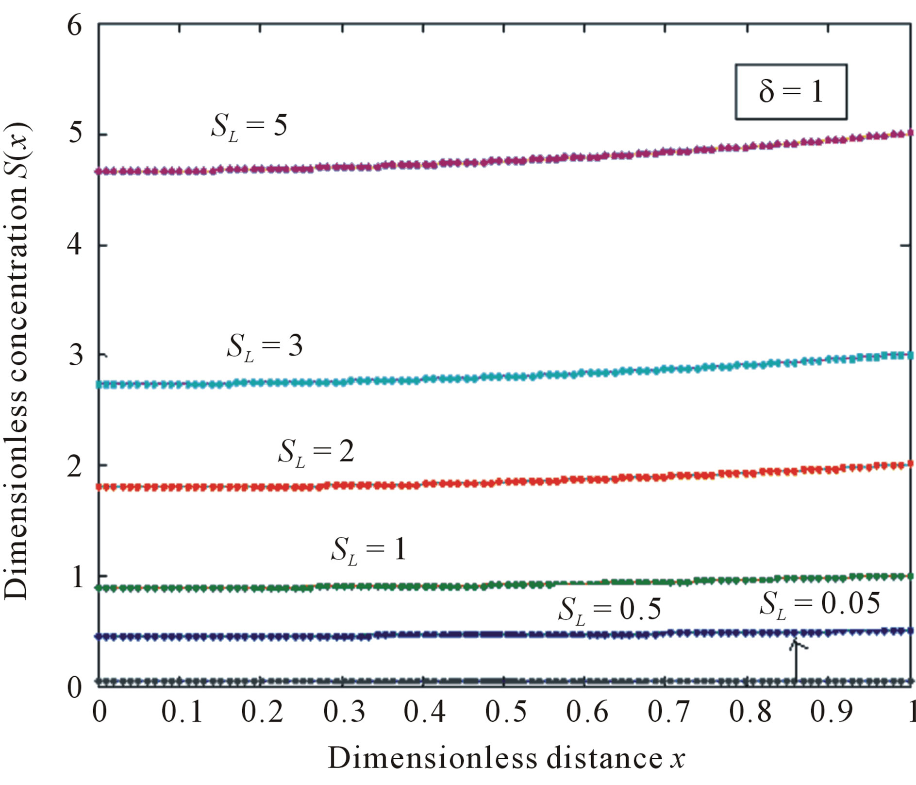
Figure 5. Normalized concentration profile S(x) as a function of dimensionless distance x. The concentrations were computed using Eq.11 for various values of the SL when δ = 1, (—) denotes Eq.11 and (…) denotes the numerical simulation.
concentration is uniform and the uniform value depends upon SL. It is clear that as dimensionless substrate concentration outside the biofilm SL increases when the value of dimensionless concentration  increases. Eq.12 represents the normalized concentration flux into the biofilm. Figure 6 represents flux versus SL (dimensionless substrate concentration outside the biofilm). From this figure, it is inferred that the value of concentration flux decreases when the thickness of biofilm increases. Figure 7 represents flux versus
 . From this figure, it is inferred that, the value of the flux is high when SL is large and then decreases slowly and reaches

Figure 6. Normalized concentration flux into the biofilm ψ as a function of dimensionless substrate concentration outside the biofilm SL. The concentrations were computed using Eq.12 for various values of the δ (—) denotes Eq.12 and (…) denotes the numerical solution.

Figure 7. Normalized concentration flux into the biofilm ψ as a function of dimensionless biofilm thickness δ. The concentrations were computed using Eq12 for various alues of the SL (—) denotes Eq.12 and (…) denotes the numerical simulation.
the minimum value when .
.
6. CONCLUSION
This paper reports a mathematical treatment for analyzing biofilm for a square law of microbial death rate. In this paper, we have evaluated a theoretical model for an investigation of the dynamic behavior of substrate consumption by a biofilm. The approximate analytical expressions for the steady state substrate concentrations for all values of biochemical parameters (δ and SL) were obtained using Adomian decomposition method. Furthermore, an analytical expression corresponding to the steady state flux response is also presented. A satisfactory agreement with the existing results is noted. This theoretical result is useful to further develop the model involving the balance of production of active biomass and bioilm erosion.
7. ACKNOWLEDGEMENTS
This work was supported by the Council of Scientific and Industrial Research (CSIR No. 01(2442)/10/EMR-II), Government of India. The authors are thankful to Dr. R. Murali, the Principal, the Mudura College, Madurai and Mr. S. Natanagobal, the Secretary, Madura College Board, Madurai for their encouragement. The author S. Muthukaruppan is very thankful to the Manonmaniam Sundaranar University, Tirunelveli for allowing to do the research work.
APPENDIX A
Basic Concept of the Adomian Decomposition Method (ADM)
Adomian decomposition method [9-13] depends on the non-linear differential Equation
 (A.1)
(A.1)
into the two components
 (A.2)
(A.2)
where L and N are the linear and non-linear parts of F respectively. The operator L is assumed to be an invertible operator. Solving for  leads to
 (A.3)
(A.3)
Applying the inverse operator L on both sides of Eq. A.3 yields
 (A.4)
(A.4)
where  is the constant of integration which satisfies the condition
 . Now assuming that the solution y can be represented as infinite series of the form
 (A.5)
(A.5)
Furthermore, suppose that the non-linear term  can be written as infinite series in terms of the Adomian polynomials
  of the form
 (A.6)
(A.6)
where the Adomian polynomials  of
of  are evaluated using the formula:
 (A.7)
(A.7)
Then substituting Eqs.A.5 and A.6 in Eq.A.4 gives
 (A.8)
(A.8)
Then equating the terms in the linear system of Eq. A.8 gives the recurrent relation
 (A.9)
(A.9)
However, in practice all the terms of series in Eq.A.7 cannot be determined, and the solution is approximated by the truncated series  This method has been proven to be very efficient in solving various types of non-linear boundary and initial value problems.
APPENDIX B
Analytical Solutions of Concentrations of Substrate Using ADM
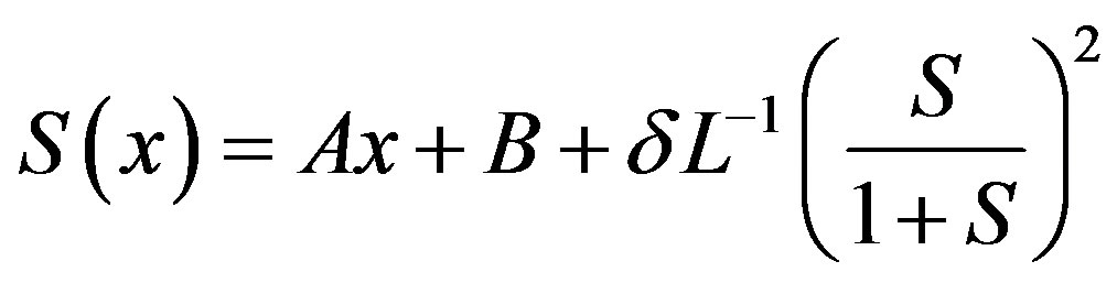
In this appendix, we derive the general solution of nonlinear Eq.11 by using Adomian decomposition method. We write the Eq.11 in the operator form,
 (B.1)
(B.1)
where  and
and . Applying the inverse operator
  on both sides of Eq.B.1 yields
 (B.2)
(B.2)
where A and B are the constants of integration. We let,
 (B.3)
(B.3)
 (B.4)
(B.4)
In view of Eqs.B.2-B.4, gives
 (B.5)
(B.5)
We identify the zeroth component as
 (B.6)
(B.6)
and the remaining components as the recurrence relation
 (B.7)
(B.7)
where An are the Adomian polynomials of  We can find the first few An as follows:
 (B.8)
(B.8)
 (B.9)
(B.9)
 (B.10)
The remaining polynomials can be generated easily, and so,
 (B.11)
 (B.12)
 (B.13)
 (B.14)
Adding (B.11) to (B.14) we get Eq.11 in the text.
APPENDIX C
Scilab/Matlab Program to Find the Numerical Solution of Eqs.7-9
function pdex4 m = 0;
x = linspace(0,1);
t=linspace(0,1000);
sol = pdepe(m,@pdex4pde,@pdex4ic,@pdex4bc,x,t);
u1 = sol(:,:,1);
figure plot(x,u1(end,:))
title('u1(x,t)')
xlabel('Distance x')
ylabel('u1(x,2)')
function [c,f,s] = pdex4pde(x,t,u,DuDx)
c = 1;
f = 1 .* DuDx;
y = (u(1)/(1+u(1)))^2;
d=0.5;
s=-d*y;
function u0 = pdex4ic(x);
u0 =1;
APPENDIX D
Nomenclature
Symbols
 : Microbial death constant, cm3/(mg day)
 : Diffusion coefficient within the biofilm, cm2/day
 : Substrate flux into the biofilm, (mg cm2)/day
 : Michaelis-Menten constant, mg/cm3
 : Biofilm thickness,cm
 : Substrate consumption rate constant, day−1
 : Dimensionless substrate in the biofilm
 : Substrate concentration in the biofilm, mg/cm3
 : Dimensionless substrate concentration outside the bioflim S1: Substrate concentration outside the biofilm, mg/cm3
T: Time, days
 : Dimensionless co-ordinates
 : Biomass yield per unit amount of substrate consumed, mg/mg
 : Co-ordinate, cm
 : Concentration of physiologically active microorganisms, mg/cm3
 : Dimensionless biofilm thickness
 : Concentration flux into the biofilm