Fractional Differential Equations with Initial Conditions at Inner Points in Banach Spaces ()
Received 12 June 2015; accepted 4 December 2015; published 7 December 2015

1. Introduction
Let  be a Banach space. We consider the nonlinear fractional differential equation
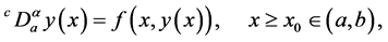 (1.1)
(1.1)
with the initial value condition at an inner point (IVP for short)
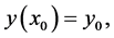 (1.2)
(1.2)
where ,
,  is the Caputo fractional derivative,
 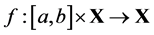 is a given function satisfying some assumptions that will be specified later.
Fractional differential equations arise in many engineering and scientific disciplines as the mathematical modeling of systems and processes in the fields of physics, chemistry, biology, economics, control theory, signal and image processing, etc. which involve fractional order derivatives. Fractional differential equations also serve as an excellent tool for the description of hereditary properties of various materials and processes. Consequently, the subject of fractional differential equations is gaining much importance and attention (see [1] - [5] ). There are a large number of papers dealing with the existence or properties of solutions to fractional differential equations. For an extensive collection of such results, we refer the reader to the monograph [1] and [3] and references therein.
In the most of the mentioned works above, the initial value problems for fractional differential equations were studied with the initial conditions at the endpoints of the definition interval, recalling that the classical existence and uniqueness theorem are for first order differential equations, where the initial conditions are at any inner points of the considered interval. On the other hand, classical integer order derivatives at a point are determined by some neighbourhoods of this point, while the fractional derivatives are determined by intervals from the endpoints up to this point. Fractional derivatives at the same point with different endpoints of the definition intervals are in fact different derivatives. Let us investigate the fractional differential equations
 (1.3)
(1.3)
and
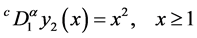 (1.4)
(1.4)
with  and the same initial value condition
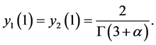
A direct computation deduces that the solutions to the above initial value problems are
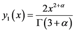
and
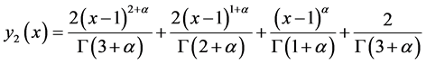
respectively. By a numerical method, we can find that  for
for . This example shows that
  and
and ![]() are two different “fractional derivatives”, and Equations (1.3) and (1.4) are two different equ- ations.
are two different “fractional derivatives”, and Equations (1.3) and (1.4) are two different equ- ations.
Motivated by the above comment, in this paper, we study the existence of solutions to the nonlinear Caputo fractional differential equation modeled as (1.1), with the initial conditions at inner points of the definition interval of the fractional derivative. In this case, the equivalent integral equation is a Volterra-Fredholm equation. Local existence results are obtained for the cases that the function f on the righthand side of the equation is Lipschitz and Caratheodory type, respectively. The theory of measure of non-compactness is employed to deal with the non-Lipschitz case. In this sense, the classical Peano’s theorem is extended to fractional cases.
2. Preliminaries and Lemmas
In this section we collect some definitions and results needed in our further investigations.
Let ![]() be the Banach space of all continuous functions
be the Banach space of all continuous functions ![]() with the norm
with the norm
![]() , and
, and ![]() the Banach space of all measurable functions
the Banach space of all measurable functions ![]()
such that ![]() are Lebesgue integrable, equipped with the norm
are Lebesgue integrable, equipped with the norm ![]() with
with
![]() .
.
Definition 2.1 ( [1] ): Let ![]() be a fixed number. The Riemann-Liouville fractional integral of order
be a fixed number. The Riemann-Liouville fractional integral of order ![]() of the function
of the function ![]() is defined by
is defined by
![]()
where ![]() denotes the Gamma function, i.e.,
denotes the Gamma function, i.e.,![]() .
.
It has been shown that the fractional integral operator ![]() transforms the space
transforms the space ![]() into
into ![]() , and some other properties of
, and some other properties of ![]() are refered to [1] .
are refered to [1] .
Definition 2.2 ( [1] ): Let![]() , and
, and![]() . The Caputo fractional derivative of order
. The Caputo fractional derivative of order ![]() of h at the point x is defined by
of h at the point x is defined by
![]()
![]() is also called the Caputo fractional differential operator.
is also called the Caputo fractional differential operator.
Lemma 2.1 ( [1] ): Let ![]() and
and![]() . Then
. Then
![]()
for![]() .
.
In recent decades measures of noncompactness play very important role in nonlinear analysis [6] - [9] . They are often applied to the theories of differential and integral equations as well as to the operator theory and geo- metry of Banach spaces ( [10] - [15] ). One of the most important examples of measure of noncompactness is the Hausdorff’s measure of noncompactness![]() , which is defined by
, which is defined by
![]()
for bounded set B in a Banach space Y.
The following properties of Hausdorff’s measure of noncompactness are well known.
Lemma 2.2 ( [8] ): Let Y be a real Banach space and ![]() be bounded,the following properties are satisfied :
be bounded,the following properties are satisfied :
(1) B is pre-compact if and only if![]() ;
;
(2) ![]() where
where ![]() and
and ![]() mean the closure and convex hull of B respec- tively;
mean the closure and convex hull of B respec- tively;
(3) ![]() when
when![]() ;
;
(4) ![]() where
where![]() ;
;
(5)![]() ;
;
(6) ![]() for any
for any![]() ;
;
(7) If the map ![]() is Lipschitz continuous with constant k then
is Lipschitz continuous with constant k then ![]() for any bounded subset
for any bounded subset![]() , where Z be a Banach space;
, where Z be a Banach space;
(8)![]() , where
, where
![]() means the nonsymmetric (or symmetric) Hausdorff distance between B and C in Y;
means the nonsymmetric (or symmetric) Hausdorff distance between B and C in Y;
(9) If ![]() is a decreasing sequence of bounded closed nonempty subsets of Y and
is a decreasing sequence of bounded closed nonempty subsets of Y and![]() , then
, then ![]() is nonempty and compact in Y.
is nonempty and compact in Y.
The map ![]() is said to be a
is said to be a ![]() if there exists a positive constant
if there exists a positive constant ![]() such that
such that ![]() for any bounded closed subset
for any bounded closed subset![]() , where Y is a Banach space.
, where Y is a Banach space.
Lemma 2.3 ( [8] ): (Darbo-Sadovskii) If ![]() is bounded closed and convex, the continuous map
is bounded closed and convex, the continuous map
![]() is a
is a ![]() -contraction, then the map Q has at least one fixed point in W.
-contraction, then the map Q has at least one fixed point in W.
In this paper we denote by ![]() the Hausdorff’s measure of noncompactness of X and by
the Hausdorff’s measure of noncompactness of X and by ![]() the Hausdorff’s measure of noncompactness of
the Hausdorff’s measure of noncompactness of![]() . To discuss the existence we need the following lemmas in this paper.
. To discuss the existence we need the following lemmas in this paper.
Lemma 2.4 ( [8] ): If ![]() is bounded, then
is bounded, then
![]()
for all![]() , where
, where![]() . Furthermore if W is equicontinuous on [a,b], then
. Furthermore if W is equicontinuous on [a,b], then
![]() is continuous on
is continuous on ![]() and
and
![]()
Lemma 2.5 ( [14] [15] ): If ![]() is uniformly integrable, then
is uniformly integrable, then ![]() is measurable and
is measurable and
![]() (2.1)
(2.1)
Lemma 2.6 ( [8] ): If ![]() is bounded and equicontinuous, then
is bounded and equicontinuous, then ![]() is continuous and
is continuous and
![]() (2.2)
(2.2)
for all![]() , where
, where![]() .
.
3. Existence Results
In this section, we study the initial value problem for nonlinear fractional differential equations with initial con- ditions at inner points. More precisely, we will prove a Peano type theorem of the fractional version. We begin with the definition of the solutions to this problem. Consider initial value problem
![]() (3.1)
(3.1)
Since the fractional derivative of a function y at an inner point ![]() is determined by the values of y on the interval
is determined by the values of y on the interval![]() , for
, for ![]() and
and![]() , we get from Lemma 2.3 that
, we get from Lemma 2.3 that
![]() (3.2)
(3.2)
The initial condition then implies that
![]()
Inserting this into (3.2) we obtain
![]()
Based on the above analysis (see [1] ), we give the definition of mild solutions to the IVP (1.1)-(1.2).
Definition 3.1: A contionuous function ![]() is said to be a mild solution to (1.1)-(1.2) if it satisfies
is said to be a mild solution to (1.1)-(1.2) if it satisfies
![]() (3.3)
(3.3)
where ![]() and
and![]() .
.
We first give an existence result based on the Banach contraction principle.
Theorem 3.1: Let![]() , and
, and![]() . Let
. Let ![]() be continuous and fulfil a Lipschitz con- dition with respect to the second variable with a Lipschitz constant L, i.e.
be continuous and fulfil a Lipschitz con- dition with respect to the second variable with a Lipschitz constant L, i.e.
![]()
Then for ![]() with
with![]() , there exist an
, there exist an ![]() with
with ![]() and a unique
and a unique
mild solution ![]() to the IVP (1.1)-(1.2).
to the IVP (1.1)-(1.2).
Proof. Since![]() , we can take an
, we can take an ![]() with
with ![]() such that
such that
![]() (3.4)
(3.4)
We define a mapping ![]() by
by
![]()
for ![]() and
and![]() . Then for any
. Then for any ![]() and
and![]() , we have
, we have
![]()
It then follows that
![]()
with![]() . Since
. Since![]() , we get that
, we get that![]() . Thus an appli-
. Thus an appli-
cation of Banach’s fixed point theorem yields the existence and uniqueness of solution to our integral equation (3.3).
Remark 3.1: The condition ![]() means that the point
means that the point ![]() cannot be far away from a. How-
cannot be far away from a. How-
ever, the following example shows that we cannot expect that there exists a solution to (1.1)-(1.2) for each![]() .
.
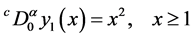
Example 3.1: Considering the differential equation with the Caputo fractional derivative
![]()
where ![]() is a constant. A direct computation shows that it admits a solution
is a constant. A direct computation shows that it admits a solution
![]()
whose existence interval is![]() .
.
However, from the proof of Theorem 3.1 we can see that if the Lipschitz constant L is small enough, then ![]() can be extended to the whole interval. Thus we have the following result.
can be extended to the whole interval. Thus we have the following result.
Theorem 3.2: Let![]() , and
, and![]() . Let
. Let ![]() be continuous and fulfil a Lipschitz con-
be continuous and fulfil a Lipschitz con-
dition with respect to the second variable with a Lipschitz constant L. If![]() , then for every
, then for every
![]() , there exists an
, there exists an ![]() with
with ![]() and a unique mild solution
and a unique mild solution ![]() to the IVP (1.1)-(1.2).
to the IVP (1.1)-(1.2).
Next we want to study the case that f satisfies the Carathedory condition. For simplicity, we limit to the case that f is locally bounded. We list the hypotheses.
(H1): ![]() satisfies the Carathedory condition, i.e.
satisfies the Carathedory condition, i.e. ![]() is measurable for every
is measurable for every ![]() and
and ![]() is continuous for almost every xÎ[a,b].
is continuous for almost every xÎ[a,b].
(H2): For every![]() , there is a constant
, there is a constant![]() , such that
, such that ![]() for a.e.
for a.e. ![]() and
and ![]() with
with![]() .
.
(H3): There exists ![]() with
with ![]() such that
such that
![]() (3.5)
(3.5)
for a.e. ![]() and any bounded subset
and any bounded subset![]() .
.
Theorem 3.3: Let ![]() and
and![]() . Assume that the hypotheses (H1)-(H2) hold, and suppose
. Assume that the hypotheses (H1)-(H2) hold, and suppose ![]() satisfying
satisfying
![]() (3.6)
(3.6)
Further assume that there exists a real number ![]() solving the inequality
solving the inequality
![]() (3.7)
(3.7)
Then there exists an ![]() such that the IVP (1.1)-(1.2) has at least a solution
such that the IVP (1.1)-(1.2) has at least a solution![]() .
.
Proof. On account of the hypothesis (3.8), we can find constants ![]() large enough and
large enough and ![]() with
with
![]() (3.8)
(3.8)
Due to the hypothesis (3.6), we can take ![]() small enough such that
small enough such that
![]() (3.9)
(3.9)
Define an operator ![]() by
by
![]()
for ![]() and
and![]() . It then follows from the hypotheses (H1) − (H2) as well as the Lebesgue dominated convergence theorem that T is well-defined, i.e., Ty is continuous on
. It then follows from the hypotheses (H1) − (H2) as well as the Lebesgue dominated convergence theorem that T is well-defined, i.e., Ty is continuous on ![]() for every
for every![]() , and that T is continuous. Further, let
, and that T is continuous. Further, let![]() . Then
. Then ![]() is a bounded closed subset of
is a bounded closed subset of![]() . For every
. For every ![]() and
and![]() , we have
, we have
![]()
due to (H2) and (3.8) which implie that![]() .
.
Below we show that T satisfies the hypotheses of Darbo-Sadovskii Theorem (Lemma 2.5). We first prove that T maps bounded subsets in ![]() into bounded subsets. For this purpose we show that
into bounded subsets. For this purpose we show that ![]() is bounded for every
is bounded for every ![]() with fixed
with fixed![]() . Let
. Let![]() . Then by (H2), for every
. Then by (H2), for every![]() , we have
, we have
![]()
It follows that ![]() which is independent of
which is independent of![]() . Hence
. Hence ![]() is bounded.
is bounded.
Next we prove that T maps bounded subsets into equi-continuous subsets. Let ![]() be arbitrary and
be arbitrary and ![]() with
with![]() . Then we have
. Then we have
![]()
which converges to 0 as![]() , and the convergence is independent of
, and the convergence is independent of![]() . Thus
. Thus ![]() is equi- continuous.
is equi- continuous.
Now we verify that T is a ![]() -contraction. Take any bounded subset
-contraction. Take any bounded subset![]() , then W is equi-continuous. So we get from Lemma 2.4, 2.6 and 2.8 that
, then W is equi-continuous. So we get from Lemma 2.4, 2.6 and 2.8 that
![]() (3.10)
(3.10)
The assumption ![]() implies that
implies that![]() , which shows that the function
, which shows that the function ![]() with
with ![]() for every
for every![]() . Hence an employment of Hölder inequality yields
. Hence an employment of Hölder inequality yields
![]() (3.11)
(3.11)
From the inequality (3.9), we deduce that![]() , which means that T is a
, which means that T is a ![]() -con- traction on
-con- traction on![]() .
.
We have now shown that ![]() that T maps bounded subsets into bounded and equi-continuous subsets, and that T is a
that T maps bounded subsets into bounded and equi-continuous subsets, and that T is a ![]() -contraction on
-contraction on![]() . By Darbo-Sadovskii Theorem (Lemma 2.5), we conclude that T has at least a fixed point y in
. By Darbo-Sadovskii Theorem (Lemma 2.5), we conclude that T has at least a fixed point y in![]() , which is the solution to (1.1)-(1.2) on
, which is the solution to (1.1)-(1.2) on![]() , and the proof is completed.
, and the proof is completed.
Acknowledgements
This research was supported by the National Natural Science Foundation of China (11271316, 11571300 and 11201410) and the Natural Science Foundation of Jiangsu Province (BK2012260).