Numerical Modeling of the Thermal Behavior of Corrosion in Conduit in Transient Mode ()
1. Introduction
The inspection of hidden corrosion at an early stage remains a main requirement in the maintenance and the repairs of deteriorated concrete structure. In fact, the degradation of concrete caused by corrosion is a very serious phenomenon which implies many risks and damages even the failure of concrete structure in civil engineering [1-3].
With the advances of NDT techniques, Infrared thermography has proven to be a good tool in detecting hidden corrosion [4], indeed (IR) thermography is widely used for non destructive evaluation of materials, especially in civil engineering and for the characterization of the heat loss in concrete structures. The thermals images obtained from infrared thermgraphy allow a quick mapping of surface structure by giving an overview of surface temperature [5-8].
In our latest works, the problem of corrosion was investigated in pipeline and oil conduit [9,10], also many defects which can occurs in concrete structure like void and cracks were studied [11,12]. The last two studies are combined on this innovative paper, hence in this work, the thermal behavior of rust layer is discussed and corrosion is detected due to a spatial-temporal structure analysis using a numerical simulation model based on FEM seen that modelling corrosion in concrete is important for predicting service life of concrete structure [13]. Therefore the use of FEM in the prediction of temperature evolution in concrete had a main importance in studying civil engineering structure.
The model of a parallelepiped concrete structure containing cylindrical conduits is adopted. This structure is supposed to be excited on the higher face by a heat flux, the lower face being maintained at a constant temperature and the other faces are supposed thermally insulated. The effects of thickness and position of the corrosion layer are studied.
2. Methods
Impulse thermography is based on the active heating of structure to be investigated, by using an internal or external heat source. The idea is that the heat transfer in materials is affected by a change in its thermal properties. Indeed, the difference between the transient temperature curves at surface above the region with defect and the one without defect is expected to provide information about the defect characteristics [14,15].
The present study gives numerical simulations of this technique using a finite element method. The aim is to verify the applicability of a thermal impulse for the analysis of the corrosion behavior in concrete structures.
When rust develops in the cylindrical structure, the steel cross-section decreases with the increase of the corrosion layer [16], which implies a lack of homogeneity in the steel section, and thus a weakening and modification physical properties (increased and reduced adhesion) [17], hence reducing the detection corrosion in this work. For reasons of simplicity, the changes in the thermal properties of materials that may occur due to chemical reactions involved in the corrosion process have been neglected in the detection of the layer thickness [18].
3. Modeling the Thermal Response
This study is undertaken on a concrete specimen (Figure 1) of (0.5 m × 0.5 m × 0.25 m), containing cylinders representing pipes, of 30.7 mm external diameter, ep = 2.9 mm wall thickness and 0.5 m length. Table 1 shows the corrosion parameters taken from [4,19] used in our model.
4. Governing Equations
The heat conduction equation of a specimen caused by Joule heating source Q is governed by the following thermal equation:
 (1)
(1)
Where:
 : is the material density (kg/m3);
 : is the Specific heat capacity (J/kg·K);
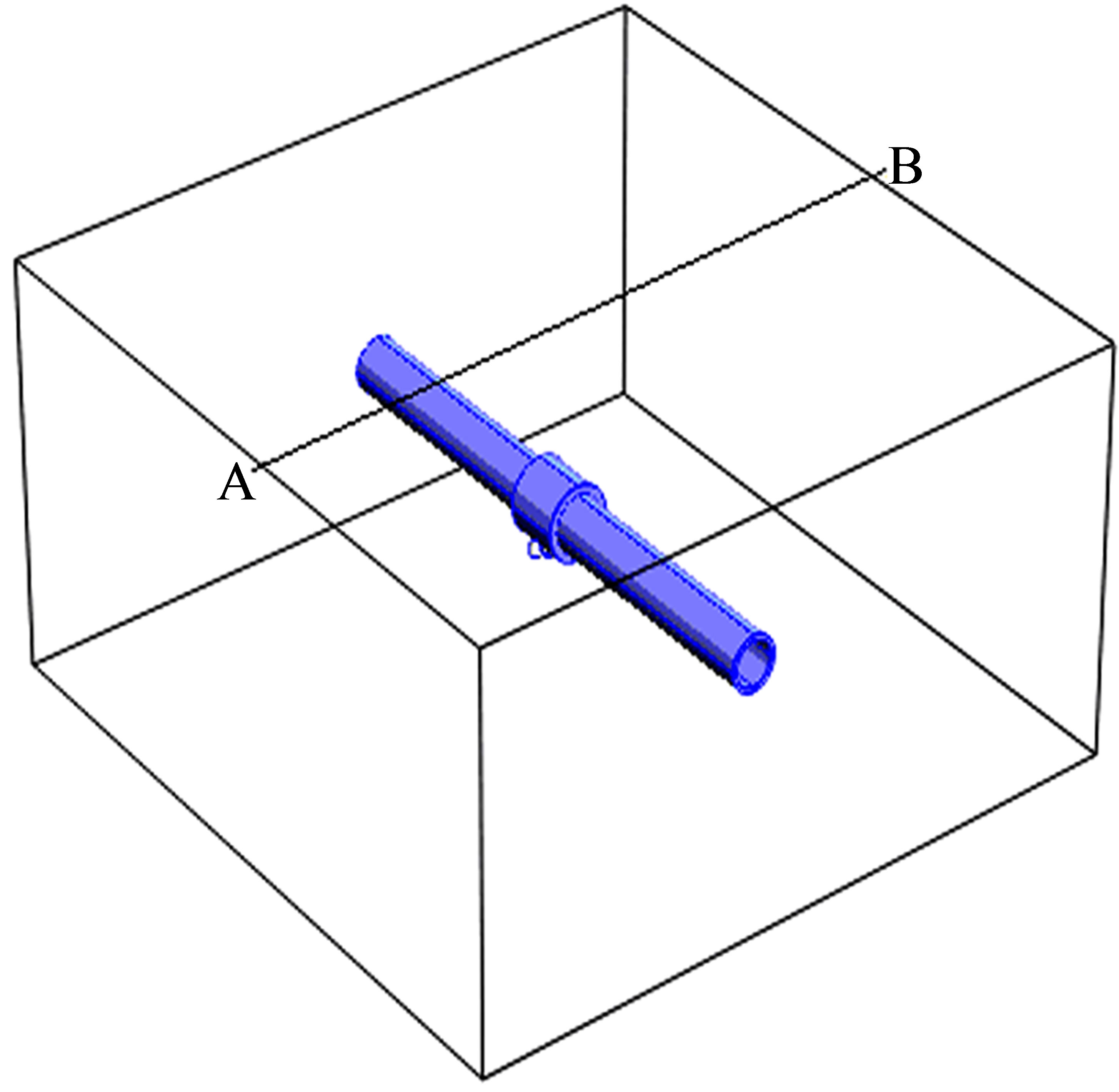
Figure 1. Finite element model of concrete specimen with defect.

Table 1. Thermal parameters of steel corrosion.
 : is the thermal tensor conductivity (W/m·K);
 : is the voluminal source of heat (W/m3).
With the boundary conditions:
 (2)
(2)
Where:
 : is the imposed temperature on a surface
 ;
;
 : is the imposed flow on a surface
 ;
;
S: is the surface of the solid;
 : is the unit vector perpendicular to S and directed towards outside.
And the initial condition:
 (3)
(3)
5. Numerical Modelling
The analytical resolution of the Equation (1) is in general inaccessible. Therefore finite element method is used for an approached solution [20-22].
The method consists in using an approximation by finite elements of the unknown functions T to discretize the variational form of the Equation (1) and to transform it into system of algebric equations of the form:
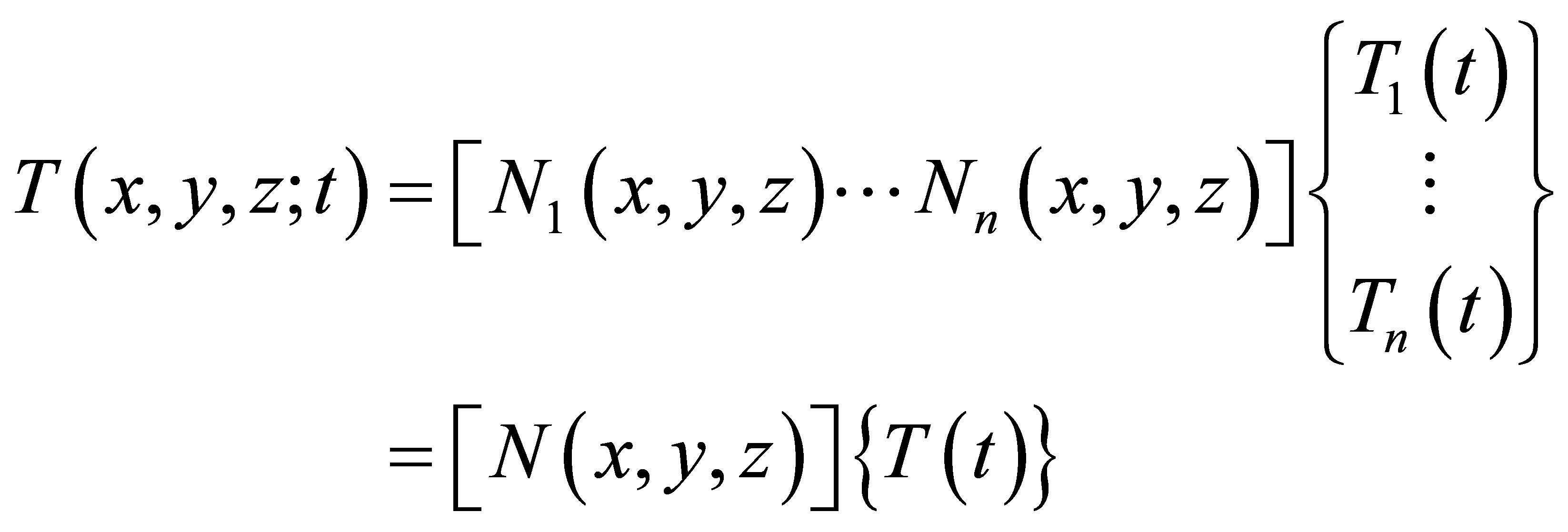 (4)
(4)
Where:
n: is the number of mesh nodes;
[N(x, y, z)]: is the interpolation matrix;
{T(t)} is the vector of nodal temperatures.
We start by building the variation form of the Equation (1). We carry out a spatial discretization which consists in calculating the elementary integrals by using finite element and a temporal discretization.
There are many softwares that can implement the method of solving finite element problems in a more or less simple and convivial way. They are interested, especially in the grid of the object studied, automatic numbering of elements and nodes, the calculation of a solution, then the results map.
In this study, we use a commercial software “Comsol” based on the finite element method and which makes it possible to calculate the temperature evolution at any moment and in any point of material [22]. The material is considered isotropic. To investigate the influence of the thermal excitation on concrete test specimen, the following boundary conditions were applied to the model [23]:
1) A thermal heat impulse is simulated, which hits the surface of the test specimen with a heat flux of 1250 w/m2, a heating time t = 900 s, and a total simulation time of 4500 s.
2) The bottom side is supposed maintained to a constant temperature T0 = 20˚C, the other sides are supposed to be thermally insulated.
5.1. Influence of Concrete Cover
The concrete cover of defect is one of the parameters that should be determined with impulse thermography measurements. To analyze the influence of this parameter, the simulation is carried out with concrete cover from 0.05 m to 0.15 m, for a rust defect having thickness er, er = 2ep = 5.8 mm (see Figure 2).
The thermographical images show the effect of the defect proximity to the input surface of the studied structure. The thermograms taken after 10 min, 30 and 60 min of cooling time (Figure 3) show only the temperature contrast of defect near the surface located at 0.05 m from the entry face. The temperature difference for 10 min is 1.2˚C, for 30 min is about 0.9˚C and 0.5˚C for 60 min of cooling time, so we can note that the suitable time to take thermograms is about 10 min of cooling time. Then, over time the effect of others defects appears gradually. This is related to the required time for heat to achieve the defect and detect it through the change in the thermophysical characteristics in the medium and translate this information at the input surface by a temperature contrast in the thermal image.
The curves of temperature versus time, Figure 4(a), show that for the three conduits; the presence of rust in conduits is translated by a drop of temperature compared to the same situation without rust. The temperature decreases when rising concrete cover. The value of the drop depends on the position of the rust in the specimen.
Figure 4(b) represents the spatial evolution of the transient surface temperature along the axis AB and re-

Figure 2. Adopted numerical model. The same defect placed at different positions in the concrete structure.


Figure 3. Thermograms recorded after a heating time of 15 min at the concrete specimen; top: cooling time 10 min; middle: cooling time 30 min and bottom: cooling time 60 min. Each thermogram was scaled to minimum and maximum.
corded after a cooling time of 10 min. During this time, there is only the effect of the rust that is closest to the surface of the specimen and that deeper rust layer does not appear well, due to the low temperature contrast, in fact the shallow pipe has good contrast after short cooling time which means that their detectability is greatly
 (a)
(a)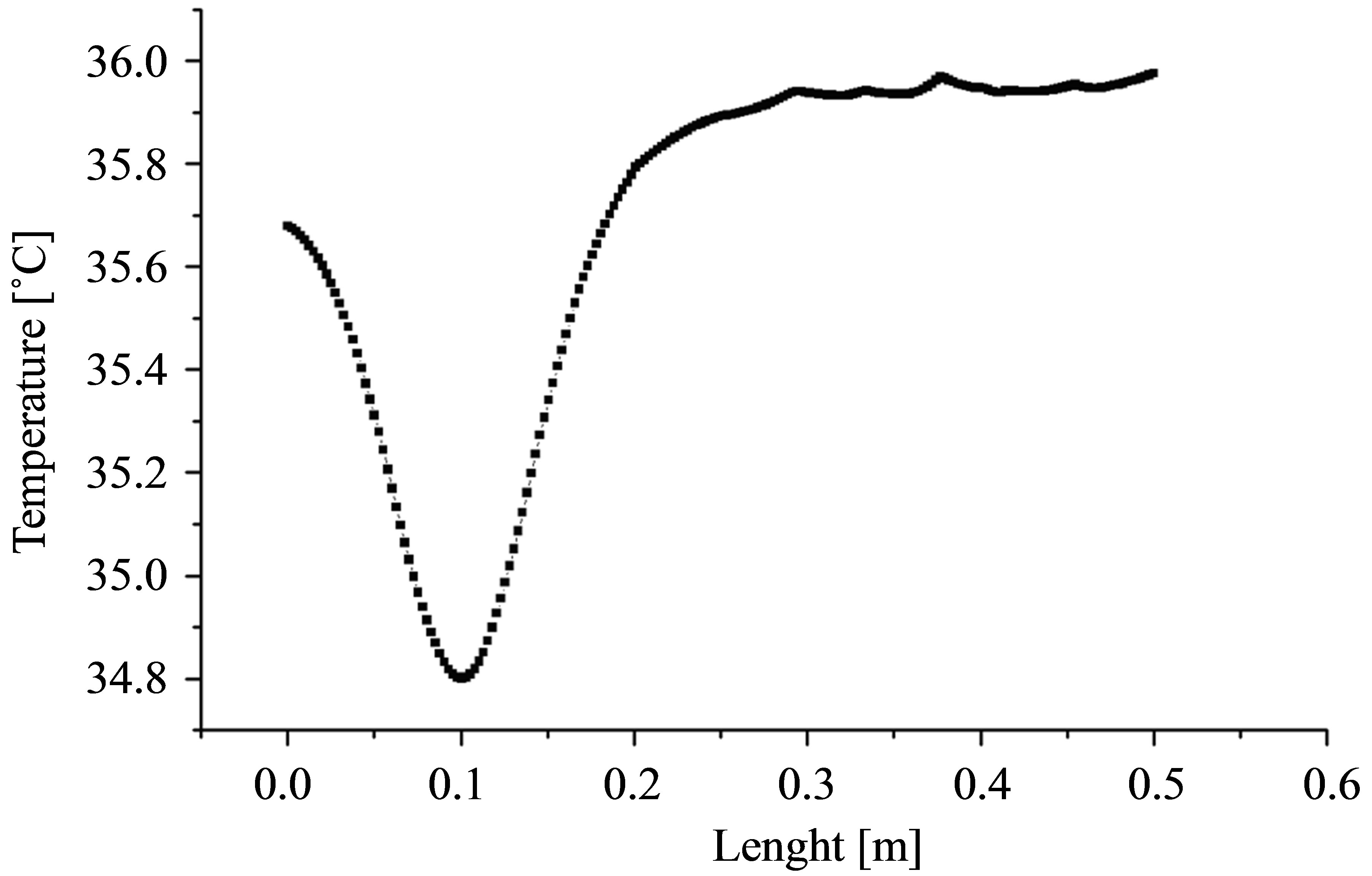 (b)
(b)
Figure 4. (a) Temperature evolution as a function of time calculated for a point taken on the center of rust surface on the three pipes and for a heating time of 15 mn. (b) Spatial evolution of surface temperature along the axis AB recorded after a cooling time of 10 min.
connected to the concrete cover.
This means that the information of the existence of the two others rusted areas has not yet the time to manifest on the surface by a temperature change. These investigations demonstrate that only the pipe in concrete up to a depth of 10 cm can appear, for those located at 15 cm it was not possible to detect them.
In order to analyze these results we represent, Figure 5, the temperature difference:
T (without rust)—T (with rust). The curves show that, to each position of the defect in the structure corresponds a minimum of this difference. When the rusted area is close to the entry surface the corresponding minimum is clear and the moment (abscissa) when it occurs is more accurate. This can give information, more accurate, on the rust position. When the rusted area is away from the input surface, the minima flattens and information on its position becomes less accurate.
5.2. Influence of Rust Size
Beside concrete cover, the rust size is another parameter affecting the thermal behaviour of rust. In this case of study, we take three different rust size, er = ep = 2.9 mm, er = 2ep = 5.8 mm and er = 4ep = 11.6 mm. For all of them the length of rust layer is 0.04 m (see Figure 6).
In the second configuration the three conduits are located at the same position by report to the sample surface, but the rust size is different from a pipe to the other.
The thermograms given in Figure 7 show that only the rust layer of a thickness er = 4ep appears with accuracy for a cooling time of 10 minutes, the other layer having the smallest thickness er = ep and er = 2ep appear when the cooling time increases. Nevertheless the temperature difference for 10 min is approximately 1.8˚C, 1.1˚C for 30 min and 0.5˚C for 60 min which means that’s the best time to take thermogram is between 10 and 30 min of cooling down.
In transient mode, the effect on the surface temperature that appears first is the region in which the thickness of the rust is the largest, task on the right in the three images. Versus time, is the effect of the average size of rust that appears and finally the smallest size.

Figure 5. Temperature difference as a function of time calculated for a point taken on the center of rust surface on the three pipes.

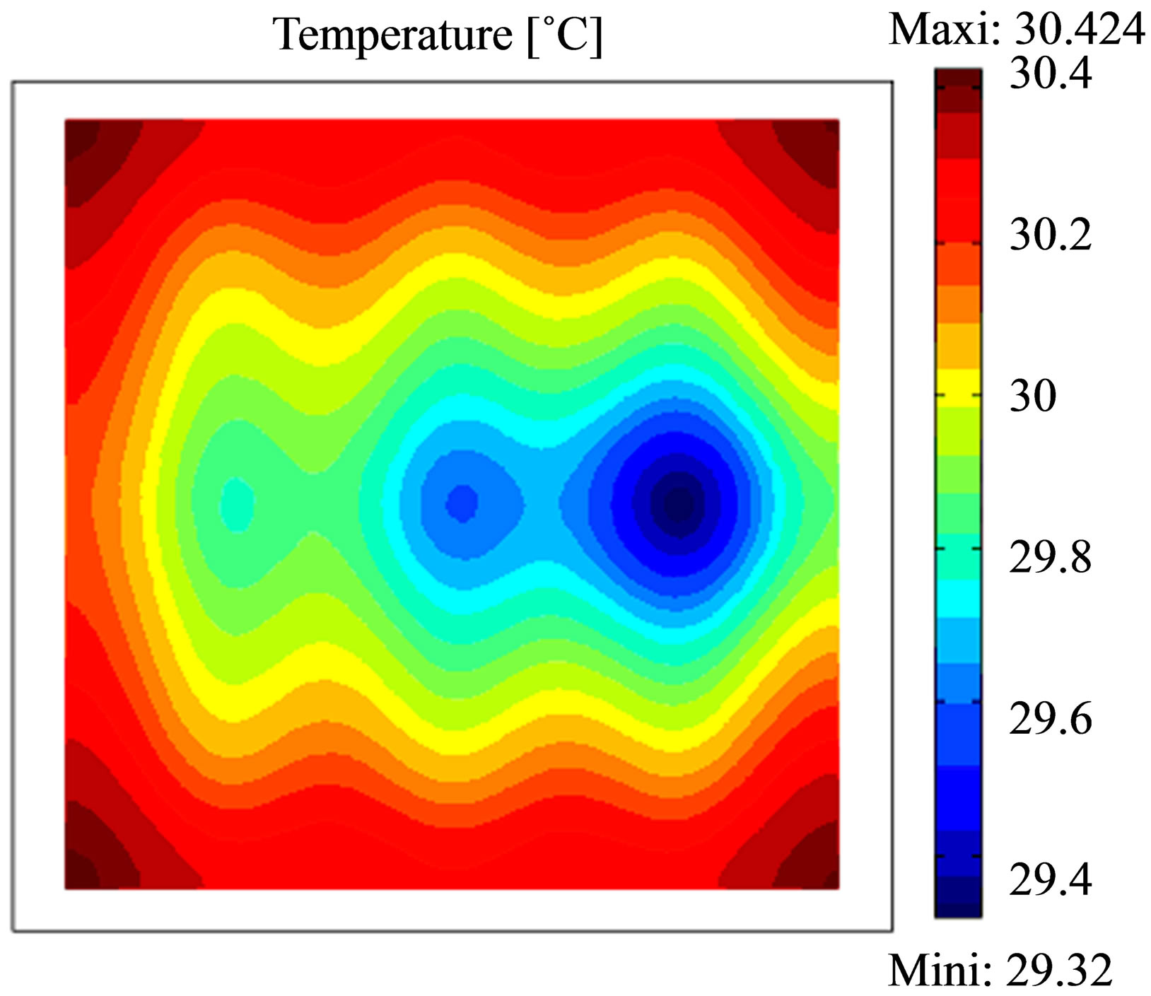

Figure 7. Thermograms recorded after a heating time of 15 min at the concrete specimen; Top: cooling time 10 min; middle: cooling time 30 min and bottom: cooling time 60 min. Each thermograms was scaled to minimum and maximum.
From these results, it appears that in transient mode, it is possible to detect the presence of different defects in the structure. Thermographical tasks, on the images, indicative of the presence of the defects are less wide in transient mode and may help to better locate them.
Figure 8(a) illustrates the temperature evolution ver-