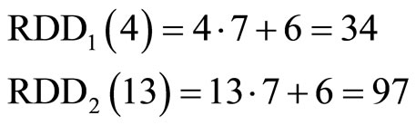
Parallel Algorithms for Residue Scaling and Error Correction in Residue Arithmetic ()
1. Introduction
Because the residue number system (RNS) operations on each residue digit are independent and carry free property of addition between digits, they can be used in highspeed computations such as addition, subtraction and multiplication. To increase the reliability of these operations, a number of redundant moduli were added to the original RNS moduli [RRNS]. This will also allow the RNS system the capability of error detection and correction. The earliest works on error detection and correction were reported by several authors [1-12]. Waston and Hasting [1,2] proposed the single residue digit error correction. Yau and Liu [3] suggested a modification with the table lookups using the method above. Mandelbaum [4-6] proposed correction of the AN code. Ramachandran [7] proposed single residue error correction. Lenkins and Altman [8-10] applied the concept of modulus projection to design an error checker. Etzel and Jenkins [11] used RRNS for error detection and correction in digital filters. In [12-16] an algorithm for scaling and a residue digital error correction based on mixed radix conversion (MRC) was proposed. Recently Katti [17] has presented a residue arithmetic error correction scheme using a moduli set with common factors, i.e. the moduli in a RNS need not have a pairwise relative prime.
In this study, we developed two new algorithms without using MRD (Mixed-radix digit) or CRT (Chinese remained Theorem) for speeding-up the scaling processes and simplifying the error detection and correction in RNS. The first algorithm is used for these purposes, through the residue digit difference cyclic property (CPRDD) within the range of , where
  with r additional moduli. The moduli
  are called the nonredundant moduli;
  are the redundant moduli. The interval,
  , is called the legitimate range, where
 , and the interval,
 , is the illegitimate range, where
 , and
, and  is the total range. This paper is organized as follows: Section II will describe the scheme the cyclic property of residue digit difference (CPRDD). Section III describes the Target Race Distance (TRD) algorithm and followed by some examples. Section IV discusses residue scaling and error correction using the TRD and CPRDD algorithms. Finally, the conclusion is given in section V.
2. Error Detection and Correction Using Residue Digit Difference Cyclic Property
Any residue digit xi representation in moduli set
 has its cyclic length with respect to its module number. For example, if the moduli set is (4, 5, 7, 9), then the cyclic lengths of any residue digits
 are 4, 5, 7 and 9, respectively. Since these cyclic lengths are not equal, they are very difficult to use as tools for error detection and correction. Actually, there exists the property of common (uniform) cyclic length in RNS between residue digital-differences (RDD). Consider three moduli set
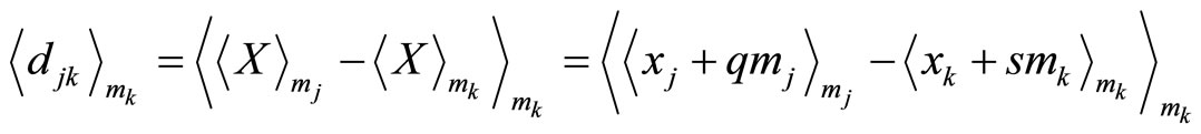
 . The residue representations and their corresponding digit-differences are shown in Table 1 and defined as the difference in value between two digits,
 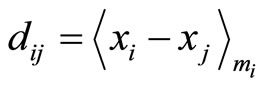 where
where  s are all modulo to positive values with respect to
  if the cycle length of
  is assigned.
Note that the residue digit-differences  in Table 1 are obtained from
  if
if , and from
  if
if . This difference of
 or
or  in values may be positive or negative, depending upon
  or
or  and
and
 or
or  respectively All negative values must be modulo to positive values. For example, on starred row 28, as shown in Table 1, the digit difference in value for
  and
and  is
is
 . It results in
From the cyclic property of residue-digit difference (CPRDD) in RNS, we now have the following theorem.
Theorem 1. For a moduli set
 and residue representation for
  in RNS, there exists a cyclic property in differences between two residue digits,
 or
or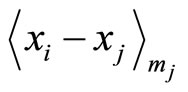 . The cyclic length can be assigned, either to
  or
or , depending upon modulo operation with respect to
  or
or .
.
Proof: Consider the case respective to , the residue-digit difference (RDD) between two digits in
 can be in general expressed by the equation
 (2-1)
(2-1)
where 

and  are integers.
For simplicity, we only consider the case of  and assume
 , and the case of
  can be obtained in a similar way.
The related theorem and algorithm are described as follows.
1) In cycle 0, (the initial cycle), we have
 with
with ,
,
 As
As 


Table 1. Cyclic property of Residue Digit Difference.
 with
with , we have
 with mj’s 0s in cycle 0, where
  means the largest integer less than or equal to x.
Thus, the RDD has mj’s “0” in the initial cycle for each modulus, i.e., in cycle 0,  for all
 .
.
2) Next consider each modulus Since
Since  and
and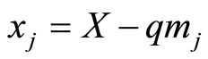 then
then
 where
where


For RDD = 0 (for cycles )
)
then

with mj’s 0 s.
For RDD = 1 (not necessary in cycle 1),
 with mj’s 1 s.
…
For RDD = mi − 1

with  s.
s.
Corollary 1. From the above theorem, we can immediately obtain that each cycle in the residue-digit difference of x will start at location 0, and end at location
 .
.
Corollary 2. It is easily shown that there exists mi number of cycles with respect to the cyclic length of .
.
Proof. Since the residue-digit difference of
 representation is pair-wise, the legitimate range of this pair-wise
  is
is , (from 0 through
 ). From corollary 1, the cyclic length is
 . Thus the number of cycles within this cyclic length for
  is
is , and for
 .
.
Theorem 2. The algorithm of theorem 1 and its corollaries can be extended to two or more pair-wise residuedigit differences.
Proof: consider a three moduli set, we have two pairwise moduli sets, whose RDD (Residue Digital Difference) is
where  is again the referenced module.
Follow the same procedure as step (2) as above.
Assume , and also pair-wise numbers
 and
and
 .
.
1) For 
thus

 “0” r2’s “
 ”
”
This shows that  has also
  “0”s in cycle 0 of
 . The cyclic length is
 , and the number of cycles for
  is
is .
.
2) For  and
and  (a constant for any RDD), if

This shows that the  in any location has also
 in cycle i of
 . The number of cycles for
  is still
 . Combining these three moduli
  into one set, we have cyclic length
  (for example,
 ). The number of cycles for
 are
are ,
,
 , and
, and , respectively. As shown in Table 1, the RDD pairs of
 , and
, and
(1, 1)
In general,  and
and
 with
with  rows and
  in each row.
This completes the proof.
Example 2-1.
Consider a moduli set ,
,  and its corresponding residue digits representation set is
 . The cyclic length is
  and the number of cycles for
 , and
, and  are
are
 , and
, and , respectively.
Error detection and correction:
Before the CPRDD algorithm used for error detection and correction is described, some basic terms in use must be defined.
Definition 1: Stride distance : It is the incremental or decremental distance between moduli
  and
and  in absolute value from ith cycle to
  cycle.
For example: .
.
(1) Error detection Let the moduli set be
 where
where  are the nonredundant moduli and
  are the redundant moduli. Since the cyclic lengths of CPRDD
  are constant, it is thus easily found that the number of cycles on track
  from the starting point 0 (or other
 ) to its target position. In turn the distance of RDD’s can also be found.
Theorem 3. The number of cycles on track  (column
 ) from any starting point (say
 ) to its target position
  can be found using the equation below;

where  the stride distance between moduli
  and
and  and k = the number of cycles passing through from starting point
  to the destination,
  on track
  If
If , then the number of cycles are equal to the total cycles from the starting point “0” to its target position
 .
.
Proof: Since  is the number of cycles from 0 to
  with respect to module
 , and
, and  is the cyclic length, thus
  is the total distance from the starting point
  to its target position
 . The remaining distance for
  on track
  in the
  th cycle must be on the same row of
  on track
 . Thus,
 .
.
Once the RDD’s of  are found, the error detection and correction for moduli can be found just by comparing the calculated cycles or RDD with the original residue representation, pair-wise so that the error module can be detected.
The procedure for error detection by using CPRDD algorithm is summarized as follows.
1) Choose two most significant (largest) moduli as the referred moduli among the n moduli, say  and
and .
.
2) Find the skip distance of a cycle
 .
.
3) Find the digit difference
 .
.
4) Create the equation of
 or
or
 (2-2)
(2-2)
5) Solve for  from Equation (2-2) as the
 and
and  are known. The value of
  must be less than or equal to
 .
.
6) Find the corresponding  distance from the starting point to
 .
.
7) Calculate  from RDD1, RDD2,
  , and check the values of
 , and …. If these sets’ numbers are equal, then no error occurs; otherwise, error exists.
We take the similar numerical as example 2-1 to verify this algorithm. (CPRDD)
Example 2-2. Assume that a moduli set
 and number X whose residue representation is
 . If an error occurs at
 , the error detection can be described as follows.
Let us begin our procedures from the
 . Since
 and
and . Then
 . Solve for
 , and let
  within legitimate range
 , then
 .
.
The corresponding  primary distances for these two
  are, respectively,
Thus, the generated results of the residue representation from  and
and  are respectively
 ,
,
 .
.
Since the calculated results of X1 and X2 are not identical, there must be errors in one of these moduli. We cannot determine which one is erroneous. To locate the module where the error exists, at least one additional (redundant) module must be used.
The procedure for error correction by using CPRDD algorithm is essential the same as the error detection. However, two additional redundant moduli  and
and  must be added for one error correction. Note that only one redundant modulus added for error detection.
1) Choose  as a referred modulus.
2) Find  as the same procedures of error detection steps 2-7.
3) Examine the values of . If common value exists among,
  then no error occurs. If there is one and only one, say
  that has no common value with all other
 , then an error exits in modulus
 . This completes the error correction procedures.
The following example is illustrated here to verify this algorithm.
Example 2-3. Error correction As before we can further locate and correct a single error by adding two redundant moduli,  and
and . Let us use the same example. The moduli set
 , where
  and
and  are redundant moduli
  and
and , and the residue X representation,
 . If a single error occurs at
 , e.g.
 , and
, and  is assigned as a reference module, then
 ,
,  ,
,  ,and
,and
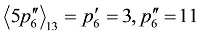
 . From CPRDD algorithm, we can find the number of cycles for these RDD’s.
 ,
,
 ,
,
 ,
,
Since the cycle length is 9, all above  values must be less than
 . Thus we have


 .
.

If no errors occur, all kij’s are equal, i.e.,
 .
.
Compared to the above results with pairwise moduli, only  meets this condition. There exists no such value in
 .
.
This shows that the module  is faulty, therefore we can correct it as follows: since
 , the
, the .
.
Thus 

 .
.
This completes the error correction.
Note that the above CPRDD’s for each residue-digit difference,  , and
, and  can be processed in parallel. In addition, if the referenced module is assigned to the erroneous module by chance, e.g.,
  this algorithm will fail to locate the error. In this case, there are no
  values that can be found to match this condition. The way to solve the problem is, of course, to assign any other moduli, e.g.,
  or
or .
.
The hardware design for the proposed algorithm in Example 2-3 is shown in Figure 1.
3. The Target Race Distance (TRD) Scheme
The conversion or decoding technique from residue representation to X in binary is usually accomplished using the mixed-radix digit (MRD) or Chinese remained theorem (CRT). An optimal matched and parallel converter of this kind can be seen in [13]. The MRD is shown by the following expression with weighted numbers:

where , and
, and  is the mixed-radix conversion (MRC) of x.
Optimization can be obtained using this method, as the accessed table lookup time is exactly equal to the right addition time, after immediate column stage for the tree network of the adders.

Figure 1. The hardware implementation for the proposed error and correction location algorithm can be accomplished without using lookup tables.
However, time is still consumed reading a large number of lookup tables. Additional hardware complexity is required by the adder-tree networks. An algorithm called the target race distance was with a simpler structure was developed for high-speed conversion.
TRD algorithm Suppose each residue number in the  has its own track
 , and the distance over track
  from 0 (starting point) to
  (end point) through
  cycles can be expressed using
 .
.
Obviously, the primary (no multiples of mi) distance of  is
is . To obtain the X from its residue representation of
 , we must find a target such that
 traversing the same distances over tracks
  respectively, i.e. when the TRD distance of each target
  is reached, then
  The TRD distance of X can be found from the following theorem:
Theorem 4. Consider the simple case of two moduli sets . Its residue representation and targets are x1 and x2 respectively. Let
  be the primary distance of residue x1 from 0 to x1 on the track
 , and
, and  be the primary distance of x2 from 0 to x2 on track
 . Then the TRD distance for these two residues x1 and x2 that have the same TRD distances can be obtained by the following equation.
 (3-1)
(3-1)
In addition, k1 can be calculated from the equation

where m1 is the cyclic length of x1, and k1 is number of cycles, all of the integers,
 .
.
Proof: It is easy to show that the above  is the common target distance of x1 and x2, Since

And thus
thus  is the TRD distances for both of x1 and x2.
Corollary: It is evident that the above theorem can be extended to n moduli set  and residue number
 . The corresponding TRD of
  are therefore

In addition, ki can be solved from the following equations.

…

where 
Note that  are the targets of moduli
 respectively and the
  is the distance that has equal track lengths, i.e.
 . That is;
 .
.
Example 3-1 Let the moduli set be
 and the residue representation be
 . The procedures to find the TRD distance can be described as follows:
1) Find the primary distance  of residue
 since
since  and
and 
is required , thus , and
, and

2) Repeat the procedure 1 to find the number of cycles k2 and k3 and the last TRD distances (destinations),
 and
and .
.
Since 


thus 
and 


thus 
and 
The final TRD distance is the common distinction of this system for targets  and
and  i.e.
i.e.
 . This result can be verified as follows:
 ,
, ,
, and
and 
Figure 2 Shows the TRD’s on tracks  and
and  respectively.
Error detection and correction by TRD algorithm A redundant residue number system with  redundant moduli will allow detection of any single error [4,14]. Consider the moduli set
 and the correct residue representation
 . Let us

Figure 2. TRD’s on track L1, L2, L3 and L4.
assume that  is the redundant moduli with a single error
  residue representation. The TRD theorem can be used to detect this error. We find that final TRD for
  and
and  does not fall into the legitimate range as follows i.e.


The final TRD distance
 . If we need to locate and correct this module error, another redundant module must be added. Let us assume that
  for this requirement in the above residue representation.
The current redundant moduli set is
 and the correct residue representation is
 . Let us assume that
  and
and  are the redundant moduli. With a single error
 . The TRD theorem can again be used to locate and correct this error. We find that final TRD’s for
  dose not fall in the legitimate range, but other final TRD’s for
  do, falls in the legitimate range:
1) TRD for  and
and 

2) TRD for  and
and 


Thus, the error is located at module m2 and must be corrected to .This algorithm can also be used for multiple error corrections. However, at least three redundant moduli are required. The procedures are similar.
4. Scaling with Error Correction
The above proposed algorithm used for error detection and correction has the advantage of not requiring lookup tables. No CRT (Chinese residue theorem) decoding processes are required. However, it is still time consuming and requires extensive hardware complexity for each module having multiple-value inputs to the match unit and selecting a correct one as a output. To improve this drawback, an optimal matching algorithm is proposed here for the error correction. The following two theorems will be used and an example follows.
Theorem 5. Let m1 and m2 be two relative prime numbers in RNS for module 1 and module 2 respectively. Then there must exist the relation represented by the equation , where
 so that
 , assuming
 . The
. The  and k are restricted to integers.
Proof: As a first step, let . It is easily seen that
  and
and  will be satisfied. Next consider
 . Since there are two different pair combination
 and
and , thus the difference between
  and
and  of k will always be satisfied for
 , where k is restricted in integers.
Theorem 6. If the values of m1 and m2 and k in the equation  are known, then p1
and p2 can always be determined from equation
 or
or , where p1p2 and k are within the range:
Proof: Let the difference value of  be equal to d, then d will be the integers within the range between 0 and m2, i.e.,
  , or
, or
 . These two expressions show that we can always select an integer value p, within the interval between 0 and
  or
or  to satisfy the conditions
  or
or 
Example 4-1 Let , and
, and . Find the minimum values of p1 and p2 respectively from the following equation :

Since  and
and , we have
 and
and
 (4-1)
(4-1)
or
 (4-2)
(4-2)
from Equation (4-1)
 so
so
from Equation (4-2)
 , so
, so .
.
This result can be verified by substituting
 into the above equation. Theorem 6 is very useful as shown in the following example.
In Theorem 3 of Section III, the number of cycles on track  from the starting point “0” to its target position “
 ” can be expressed by setting
 , i.e.
 (4-3)
(4-3)
where  is the module i stride distance referring to module j. Similarly, the number of cycles on track
  from the starting point ”0” to its target position “
 ” can be expressed by setting
 , i.e.;
 (4-4)
(4-4)
Since, from theorem 3, the cyclic length of the residue digits differences reference to module mj is constant (uniform), then there must exist a condition,
 Eliminating the above terms from Equations (4-3) and (4-4),


where ,
,  and
and

Example 4-2 Let the moduli set 
 , and the error
 , the error occurs at m3.
Follow the same procedures of the Example 4-1 to use this algorithm.
 (4-5)
(4-5)
 (4-6)
(4-6)
 (4-7)
(4-7)
 (4-8)
(4-8)
Eliminating  and
and  from Equation’s (4-5) and (4-6)
 ,
,

solve for  from (4-5),


or 

 .
.
Check from Equation (4-5),


This shows that the error occurs at module m3. From this result, we can immediately obtain . Noting that it may happen that the assigned referenced memory moduli falls coincidentally with error memory module m3. In this occurrence, we cannot find the correct (integers) values of P1 and P2 within the legitimate range. It seems that this algorithm can only detect error. To complete the error correction procedure, we can simply change the referenced module to any other and follow the same procedure as before. This guarantees that the proposed algorithm in Theorem 4 will also work well in this case. The hardware structure for illustrating this algorithm is shown in Figure 3.
The proposed TRD (target Race Distance) scheme used for error correction can be used for scaling and assigning numbers in a residue number system. A redundant residue number system (RRNS) is defined as before in an RNS with r additional moduli. The moduli
 , are called the nonredundant moduli, while the extra r moduli,
  are the redundant moduli. The interval,
  , is called the legitimate range where
  and the interval,
  , is the illegitimate range, where
  is the total range. In the RRNS, the negative numbers within the dynamic range are represented as states at the upper extreme of the total range, which is part of the illegitimate range. The positive members are mapped to the interval
 , if Mk is odd, or
 , if Mk is even. The negative numbers are mapped to the interval

Figure 3. In the block diagram using optimal matching between multiples Pi m and Pkmk, the residue digits are corrected by xi - x4 = di4.
 if Mk is odd or
 if Mk is even [14].
The one-to-one correspondence between the integers of the dynamic range and the states of the legitimate range in the RRNS can be established using a polarity shift. [11], The polarity shift is defined as below.

where  denotes the value X after a polarity shift and
 if
if  is odd, so that
 a polarity shift needs to be performed prior to correcting or scaling since
  belongs to the legitimate range. If a single residue digit error
  is introduced and corresponds to modules mj, then, after a polarity shift.

where  is the multiplicative inverse of
  moduli mj i.e.
  and
and  The
The 
denotes a single residue digit error and must fall within the illegitimate range ,  [11].
[11].
Since , and can be represented uniquely by
 ,where
are the coefficient from the Chinese Remainder Theorem
(CRT), i.e,  , where
 . Note that the redundant digits
  are zeros if no error is introduced, while at least one redundant digit is not equal to zero if a single error is introduced. Therefore, it has the same meaning that
or  is used to be the entries of the error correction.
1) 2)
2) 
Although the errors detection and correction described in section II have been simplified the processes due to no need of CRT conversion. It is still hardware complex and time consuming for the residue scaling operation. To improve this drawback, a direct residue-scaling algorithm can be used. It is flexible and direct to detect and prevent the errors. The flexibility means that the scaling factor can be arbitrary chosen any single module such as , i.e. not necessarily beginning from
  to
to . in order. The direct capability means no requirement for CRT extension processes for decoding or lookup tables. The following theorem (theorem 7) and example are clarified.
Theorem 7. If the scaling factor K is one of the module set  and the residue digits are
 , respectively, then the residue digit
  scaled by a factor
 can be obtained using the equation
 (4-9).
Proof: It is easy to show that when , and Equation (4-9) is divided by
  on both side, we have
 (4-10).
Example 4-3. For convenient comparison of the proposed TRD algorithm to other schemes such as appeared in [14], we take the same numerical example in [11]. Let the moduli set , where
  are regular moduli and
 are redundant moduli. Then
 ,
,  ,
,
 , and
, and
 . The sufficient conditions for correcting single residue digits errors are 1)
 , or 4,
  , or 2,
 , The maximum
 , and 2)

Thus the moduli set satisfies the necessary and sufficient conditions for correcting single errors digit. Assume  and a single digit error
  is introduced, then
 .
.
After a polarity shift, 
Follow the same procedures as shown in Example 4-2. CPRDD is applied for correction without the need for using a table.
1) Assign the moduli  as the reference moduli, the following residue digit references and its corresponding CPRDD equations:
  are obtained


2) Choose two highest digit difference as one pair for equal target race distance e.g.
 . Then the true primary RDD equations are
 (4-11)
And  (4-12)
where  and
and  are selected so that the two RDD are equal distances.
3) Eliminating k terms in Equation’s (4-11) and (4-12) by putting 

 where
where
 , then
 .
.
4) Substituting p1 and p2 into equations (4-9) and (4-10) respectively, we have , then
 , and
, and , also,
 .
.
5) Checking other three RDD’s


The only different module residue occurs on module number at , i.e.,
 . The three target distances, can be from any module residue, say, (except
 ),
), .
. .
.
The residue representation of X is therefore,
 . If a single digit error
  is introduced, then,
 .The corresponding error is therefore


After a polarity shift,
and the scaling factor  to
to  is
is
 . The final step must use a lookup table to obtain the result,
  [13].
[13].
For verifying our proposed algorithm, the table of the corresponding  is not required as in [13]. The processes for finding and correcting a single error based on our method are described below.
1) Find the residue digit difference to a selected module, say  as before
 . For verifying that our proposed algorithm detects and corrects single error without using a table, the same numerical example is used to describe the procedure as follows:
 ,
,
 ,
,


Then


2) Choose two highest digit differences as one pair for equal target race distances. e.g.
 and
and , the following two equations can be obtained:
 (4-13a)
 (4-13b)
3) Eliminating k terms in (4-13a) and (4-13b) by putting 
 then
then  and
and .
.
4) Substituting  and
and  into Equation’s (4-13a) and (4-13b) respectively, we have
 , then
 , and
, and , also,

Obviously, the error is located at  thus
thus
 .
.
Furthermore, the CPRDD algorithm can be used directly and in parallel for residue scaling and error correction. Thus the process is greatly speeded up.
Example 4-4 For convenient comparison, the same numeric example as in [13] is illustrated here. Consider , and scaling factor
 . If an input
 and a single residue digit error
 , corresponding to
 Then
Then 
After a polarity shift,

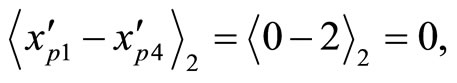
1) Dividing by  after subtracting
  from
from 
 , this leads
 ,
,
 ,
,
 ,
,
 ,
,
 .
.
2) Dividing by  after subtracting
 from
from 


Since from above only k3 does not match with all other’s ki, i.e.  and
and . Therefore, there occurs an error at
 . Once this error is detected, it is easily found and corrected from the above equations,
  , which in turn
 and
and .
.


that 
Divided by “2”,


 .
.
Divided by “5”
 ;
;


 .
.
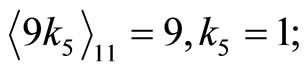
The hardware structure of this example for the residue scaling is shown in Figure 4.
Actually this algorithm can be divided by any arbitrary moduli.
Example 4-5 Divided by any arbitrary moduli, say , it must subtract
  from X


Then


check .
.
This results


It can be seen from above that
 which are equal each other as expected.
Example 4-6 For processing two residue scalings and error corrections in parallel, we take Example 4-4 as an illustration. Let scaling factor , i.e., the first residue scaling factor is 2 and the second one is 5 or verse versa. It is easily shown that the extended CPRDD algorithm is used and can be completed in one cycle. That is


The result is identical
 , i.e.,
 , and
, and , which are identical results as shown in Example 4-4.
Example 4-7 For error correction


Figure 4. Hardware structure of the residue scaling number for Example 4-4.


the correct 

 , and
, and

This shows . Therefore the error correction is made by
  and
and
 , which corresponds to the value in Example 4-4, in scaling factor
 , (dividing by “5” part).
From above results, this checks that scaling
 which is within the accuracy of the residue scaling factor.
In a general case,  , this time we must modify the subtraction of
  and
and  from the X, before the process of the scaling. If
  is the scaling factor, then the subtraction must change to
 , where
  so that
 or
or  Let us consider the following example:
Example 4-8
 of moduli set
 . The scaling factor
 . is assumed. Then, residue
 , and
, and  can be found from
 .
. . Thus
 and
and .
.
Alternatively, it could be from other module ,
,  , where
 and
and


 which has the same number to be subtracted.


From CPRDD algorithm, the scaling processes are performed as before, we then have the following results by scaling factor ;
;


Thus , which is exactly the value
  and is the most closed to
 .
.
This result can be checked using sequential steps as follows:
For 


Divided by 2:


30 0 811 Divided by 7:


This result of  shows that the CPRDD algorithm has the capability of parallel processing operations in residue scaling and error corrections, i.e., any combination moduli scaling factors for Ks of moduli set {m1, m2,
  , mk} can be performed simultaneously.
5. Conclusions
The arithmetic operations in the residue number system for addition, subtraction, and multiplication can be speeded up by using its parallel processing properties. However, some difficult operations, such as error detection and correction, must go through conversion or decoding processes from the residue representation to the regional binary number x. This is because the decoding technique is usually accomplished using the mixed-radix digit (MRD) or Chinese Remained Theorem (CRT), which are time consuming processes requiring hardware complexity. We proposed two algorithms for scaling and error correction without the need for lookup tables or increasing the encoding process.
The Cyclic property of the Residue-Digit Difference (CPRDD) algorithm can detect and correct errors from the RNS cyclic property. Any residue moduli set has a specific cycle length, which can be obtained from the individual residue number, difference, each pair, to a reference memory module mi. Once the cyclic length is known, then the original value x is easily found, and in turn, the errors can be detected and corrected.
The TRD (Target Race Distance) algorithm combined with CPRDD is used for scaling and for error detection and correction. The scaling results and error correction can be directly performed by these two algorithms without using MRD or CRT. Thus, the decoding process is significantly reduced, and the hardware structure is greatly simplified. Several examples are illustrated and verified for these two algorithms.