Semi-Implicit Scheme to Solve Allen-Cahn Equation with Different Boundary Conditions ()
1. Introduction
Allen-Cahn equation was introduced by Allen and Cahn [1] [2] and can be viewed as a simple model to study the phase separation, such as ferromagnets with positively and negatively magnetized domains and viewed as a reaction diffusion equation in material sciences. The Allen-Cahn equation is a nonlinear kind of the heat equation. Similarly, to the heat equation, it contains a term that tends to make the field constant, given by a Laplace operator accomplishing a local average around any fixed point, and send this average towards zero. Many methods can be used to solve nonlinear PDEs. In [3], the author use Adomian Decomposition Method coupled to the Lesnic’s approach to solve boundary value problems and initial boundary value problems with mixed boundary conditions for linear and nonlinear partial differential equations. Allen-Cahn equation has been applied to many problems, such as image analysis [4] [5] the motion by mean curvature flows [6]. In particular, it has become a essential model equation for the diffuse interface technique proposed to study phase transitions dynamics in materials science [7]. Furthermore, an efficient algorithm of this equation has proposed. Several numerical schemes have been suggested to solve Allen-Cahn equation, and including the finite difference method, the finite element method. In [8], the authors propose some efficient and accurate numerical methods to compute the steady-state of variable coefficients space fractional Cahn-Allen equations. The approach combines an adaptive time stepping semi-implicit gradient flow method to minimize the fractional energy functional and pseudo-spectral approximation schemes. Based on the use of a preconditioned GMRES, the space fractional Cahn-Allen equation is then solved efficiently. In [9], the author proposed and analyzed for the Cahn Allen equation by dividing the equation into linear part and nonlinear part based on the idea of operator splitting. For the linear part, it is discretized by using the Crank-Nicolson scheme and solved by finite element method. The nonlinear part is solved accurately.
In [10], the authors split the Allen Cahn equation into the linear heat and nonlinear equations; and then solve the linear part using the Fourier spectral method and the nonlinear part using an analytic closed-form solution. These steps are unconditionally stable. However, if a large time step is used, then the nonlinear part dominates the evolution and results in a sharp interfacial transition layer.
In this paper, we will look at the two dimensional form of the Allen-Cahn Equation corresponding to Equation (7.9) in [11] with
and
, where
satisfies
(1)
supplemented with the Dirichlet or Neumann boundary conditions and the initial conditions
(2)
Here
. Here, f and g are two given functions, that will be fixed later for numerical study. It is a parabolic, nonlinear and nonhomogeneous PDEs in two dimensions. Moreover, the parameter
is the time and
is a parameter to fix, which can small leading to a stiff problem (and possibly unstable discretization schemes). To get a well-posed problem, we need to add a boundary condition on the boundary of the domain, i.e.
, that we choose as the non-homogeneous Dirichlet boundary condition
on
. Finally, since we have an initial value problem, we provide an initial data
in
. Many numerical simulations of Allen-Cahn equation was presented, see [11] [12] for a non-exhaustive list. The paper is organized as follows. In section 2, we recall some properties related to five points approximations of
and the tensor product that will be used in our MATLAB code. In section 3, a semi-implicit finite difference will be formulated for homogeneous Allen Cahn equation with Dirichlet boundary condition. In section, 4, a semi-implicit finite scheme for homogeneous Allen Cahn equation with Neumann boundary condition will be presented. In section 5, we will consider the Non-homogeneous Allen Cahn equation with Neumann boundary condition as good application to valid our numerical approach, numerical tests will be presented for different choice of initial data to validate our algorithms and our code of calculation. Then we conclude.
2. Preliminary
We consider the square domain
, discretized by N segments in each direction x and y. The number of interior points is
, and the total
number of interior points is
. The discretization step is
. The
boundary
is discretized by using 4N points. The boundary is composed of four parts
, for South, West, North, East.
If ones considers a Dirichlet boundary condition, then we have
on the boundary
for solving the Laplace equation
in
. We recall that under a suitable mathematical setting, the well-posedness of the problem can be proved. For the interior points, we use a five points stencil approximation of the negative Laplacian
(3)
on the square lattice
with Dirichlet boundary condition
on the boundary grid points [13] [14] [15]. In addition we have a right hand side (rhs)
. The corresponding matrix
of the Laplacian is computed by using (3) for the interior points, resulting in a
positive definite matrix. Nevertheless, in the case where Equation (3) holds for a point
where one of the points with index
,
,
,
is on the boundary, one must use the fact that we now the boundary value. As an example, if one writes Equation (3) for
, then the point
is on the south boundary and we have
. This directly implies that considering Equation (3) one gets, for
,
If one assumes that
or m, then we have
For the corner’s points, we must also handle the value of the left (
) and right (
) endpoints. From above, we see that the matrix is modified as well as the right-hand side. Globally, the approximation of the Laplacian with Dirichlet boundary condition leads to solving a linear system that we latter write
.
The resulting matrix
is sparse, positive definite and of size
. Let us remark that the above system can be solved efficiently by using a LU factorization or any well adapted linear system solver. In practice, the matrix
can be built in MATLAB by a tensor operation, based on the function kron as
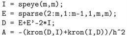 (4)
(4)
Here, kron is the Kronecker Product function computes the Kronecker tensor product of two matrices, more precisely if we have two matrices A and B the Kronecker tensor product is defined as:
then
3. Discretization for the Dirichlet Boundary Condition
3.1. Semi-Implicit Backward Method: System of Non-Linear Equation
Semi-implicit finite difference schemes are used for the Allen Cahn equation. Namely, the time derivative is approximated by the backward-Euler and a second-order backward differentiation formula scheme is applied for the Laplacian operator (see Equation (3)) whereas the semi-implicit technique is used to deal with nonlinear part. This means we write all the terms implicitly except for the nonlinear term which is treated explicitly. Let
be the node spacings in the x and y directions and
is the step time. If we denote by
, here i, j is location node numbers, k is the time time step number, then after discretization get
(5)
with initial condition:
and boundary condition:
Rearranging the Allen Cahn equation
(6)
For simplicity, we can assume
we have the final form of discretized Allen Cahn equation
(7)
In the next subsection, a more compact form of Equation (7) will be presented.
3.2. Semi-Implicit Method: Matrix Formulation
Concerning the discretization, use a uniform time step
and a uniform spatial discretization size h in both the x- and y-directions. We call
the matrix that represents the five points stencil discretization of the 2D negative Laplacian (
), given by Equation (3), on the square lattice
with Dirichlet boundary condition
on the boundary grid points. These values are directly replaced into the system since they are given values. The matrix
is therefore a positive definite matrix of size
, where
is the number of interior grid points. Since we use a inhomogeneous Dirichlet boundary condition, and will have a right hand side
latter related to a source, we denote by
the modified right hand side based on the inhomogeneous boundary condition and the five points stencil discretization of the Laplacian.
The nonlinearities in the PDE are trivial (
) to deal with if we choose an explicit time integration method for the nonlinear part and backward time integration for the linear part, all the mathematical details for the nonlinear discretization of Allen Cahan equation is presented in subsection 3.1, we call this method a semi-implicit backward scheme.
If we choose an explicit time integration method for Allen-Cahn equation, such as the Forward Euler finite difference, there is a strict restriction on the time step size to get convergence, for further details see [16]. Since the problem is a nonlinear dynamical system, for stability reasons, we propose taken explicitly a semi-implicit backward Euler scheme with the nonlinear part (as presented in subsection 3.1).
Reorganizing the equation gives a PDE for
(see Equation (7)), leading then to the following linear system for each time step
,
(8)
where I is the identity operator and A is the discrete two-dimensional matrix for
(see Equation (4)), with initial condition
and with the inhomogeneous boundary condition
on
, and the boundary condition becomes
The right-hand side
must be updated at each time step for evolving the nonlinear system. When passing at the full discretization (both in space and time), then one gets the following linear system at each time step
to solve
(9)
for the interior grid points. The matrix
is the identity matrix of size
.
3.3. Solvers
When solving (9), we need to solve a sparse positive definite linear system at each time step. For the project, we coded a LU factorization after entering the time loop, to optimize the system solution. In addition, we also wrote Jacobi and Gauss-Seidel iterative methods that work well since the linear system is positive definite [17]. The linear system solution is fast and provides a real-time evolution of the solution. Finally, concerning the post-processing, we plot the solution onto the square at each time step.
3.4. Example
In our numerical example, we take the initial data
(10)
and we work with the Dirichlet boundary condition
.
• We will use the Gauss Seidel iterative method to compute the solution of the matrix equation. For that, we fix the tolerance (tol) = 10−6 and we compute the discrete solution until the stopping criteria is verified. Figure 1 and Figure 2 represent the discrete solution obtained via Gauss Seidel iteration method. The error term in Gauss Seidel iteration is defined as the difference between two consecutive iterate and more precisely our stopping test based on
. The circle shrinks with time and disappears.
![]()
Figure 1. Solution using Gauss Seidel iteration method at different times.
![]()
Figure 2. Numerical solution of Allen Cahn equation at different times.
• Like the Gauss Seidel technique, the Jacobi method is considered to solve the matrix equation associated with the Allen Cahn equation. The same phenomena is observed.
• Since, the algorithm proposed is a semi-implicit finite difference, there is no restriction on
and h to get convergence. In our numerical implementation, we tested different choice of
and h. For practical simulation, we take a small space step size
and a time step
. Moreover, the epsilon parameter is chosen very small,
.
• The changes in the circle over time are shown, in Figure 1, Figure 2 with
,
,
. The inner circle has a larger curvature, it shrinks faster than the outer circle, and after the inner circle disappears.
4. Discretization for the Neumann Boundary Condition
4.1. Goals
A second variation concerning the problem consists in considering a homogeneous Neumann boundary condition at the interface
. We can expect then a very different behavior of the numerical solution because of this fundamentally different boundary condition. Basically, the main point that must be modified is the way the discrete Laplacian matrix is computed. Here we call this matrix
, which is of size
. To approximate the normal derivative, we use the approximation
for the west side of the square, i.e.
(the extension to the three other sides is trivial). When considering the five points stencil approximation of the Laplacian at point
(except at the upper and lower left corners)
(11)
then, since
, this simplifies as
(12)
For the Neumann boundary condition, the right hand side
is an element of
. The source term is built from the right hand side of Equation (8) at the discrete points. Finally, we have to solve a linear system in the form
(13)
for the interior grid points. This can clearly be done as for the Dirichlet case, i.e. by a LU factorization (the one which is coded here), a Jacobi or Gauss-Seidel fixed point iteration. We have only retained here the LU factorization from the numerical study performed for the Dirichlet situation. Indeed, the LU factorization is done only once before entering into the time loop, and then a forward-backward substitution is applied at each time step at a cost
. The L and U matrices remain with a low bandwidth because of this property on
(as well as
).
4.2. Example
In our numerical example, we take the initial data (10), namely
(14)
• We set a homogeneous Neumann boundary condition
, where
is the square domain
.
• Using Direct method and considering a uniform step-size
and the time step
.
• Figure 3(a) shows the graph of initial condition given by Equation (10).
• The large-time behavior of solutions to Allen Cahn equation is established numerically for initial condition given by Equation (10). It’s observed that the circle shrinks slowly with time and disappears, see Figure 3(b).
![]()
Figure 3. Allen Cahn problem with homogeneous Neumann boundary condition and
.
If we solve the Allen Cahn equation with
with homogeneous Neumann boundary condition, the solution is unstable It’s necessary that
, for further details see [18]. So taking
and
, the scheme explodes and is unstable.
5. Non-Homogeneous Allen Cahn Equation with Neumann Boundary Condition
5.1. Formulation and Discretization
Considering the Non-Homogeneous Allen Cahn equation:
(15)
where g is a given function and supplemented with the homogeneous Neumann boundary conditions
(16)
and the initial conditions
(17)
Here
. The same strategy applied for homogeneous Allen equation and more precisely using Equation (7), we deduce that:
where
.
5.2. Numerical Results
In our simulation we consider two different initial conditions: the first one is given by Equation (10) and the second one is given by (18)
![]()
Figure 4. Neumann condition: Contour of discrete solution (CDS) for Allen Cahn equation at different times.
![]()
Figure 5. Contour of discrete solution (CDS) at different times. The straight line move to the right.
(18)
For numerical implementation, we consider
. We make different numerical tests to see how the initial data and the function g has an effect on the behavior of the solution.
1) Considering the space domain (‒5, 5)2. If one consider as initial data (10) and
it’s observed that the circle grow instead of shrink as in the case of
, see Figure 4.
• Considering the case where
, and using Equation (18) as initial condition the line curve move to the right direction, see Figure 5.
![]()
Figure 6. Contour solution at different times. The straight line move to the right and become curved.
• Note that of
, one can that the line curve move to the left direction.
• Considering the case where
, the straight line move to the right and become curved, see Figure 6.
6. Conclusion
Using finite difference method, we can solve nonlinear PDEs, more precisely we have obtained a numerical solution to the Allen Cahn equation. We have formulated using semi-implicit finite difference method and coded the corresponding algorithm to the Allen-Cahn equation. Three methods were used with the Allen-Cahn equation: the Direct method, the Jacobi and Gauss-Seidel iteration Methods. For small mesh size and small-time steps, it is better to use iterative methods, since the size of the matrix will be very large. Dirichlet boundary condition is considered, the solution is obtained and analyzed sing Direct and iterative technique. We also solved the Allen-Cahn equation using homogenous Neumann boundary conditions, this involved using ghost points next to the boundary. In the case of Neumann boundary condition the circle with
grow instead of shrink as in the case
. Moreover, for Neumann boundary condition, if we consider an initial data set
for
and
for
. If you take
nothing was happened, but if we take
the line move in the right direction and if you take
, the line move in the other direction (left direction). Considering the case where
, the straight line moves to the right and become curved. All the numerical tests confirm that the initial data and the function g has an effect on the behavior of the solution. All the methods presented were coded using MATLAB.