Study for System of Nonlinear Differential Equations with Riemann-Liouville Fractional Derivative ()
1. Introduction
Let  denote the
  matrix over real fields
  or complex fields
 . For
. For 

here  is the usual space of continuous functions on
  which is a Banach space with the norm

The space  is defined by

(see [1]).
The existence of solution of initial value problems for fractional order differential equations have been studied in many literatures such as [1-4]. In this paper, we present the analysis of the system of fractional differential equations
 (*)
(*)
where  denotes standard Riemann-Liouville fractional derivative, where


 and
and  is a square.
To prove the main result, we begin with some definitions and lemmas. For details, see [1-5].
Definition 1.1 Let  be a continuous function defined on
  and
and . Then the expression

is called left-sided fractional derivatives of order 
Definition 1.2 Let  be a continuous function defined on
  and
and  Then the expression

is called left-sided fractional integral of order 
Lemma 1.3 Given  with eigenvalues
 in any prescribed order, there is a unitary matrix
  such that
  is upper triangular with diagonal entries
 That is, every square matrix
  is unitarily equivalent to triangular matrix whose entries are the eigenvalues of
  in a prescribed order. Further more, if
  and if all the eigenvalues of
  are real, then
  may be chosen to be real and orthogonal.
Lemma 1.4 Assume that  with fractional derivative of order
  that belongs to
 . Then

for some  When the function
  then
then
 where
where
 and
and 
Lemma 1.5 (Schauder’s fixed theorem) Assume  is a relative subset of a convex set
  in a normed space
  Let
Let  be a compact map with
 . Then either
(A1)  has a fixed point in
 , or
, or
(A2) there is a  and a
and a  such that
Now, let’s us give some hypotheses:
H1:  is continuous on
  and is such that
 (1)
(1)
where  is a continuous function on
H2:  is continuous on
  and is such that
 (2)
(2)
where  is a continuous function on
Lemma 1.6 Let  If we assume that
  then the initial value problem
 (3)
(3)
where


has at least a solution  for
for  sufficiently small.
Proof. If
 then
then , by Lemma 1.4, We are therefore reduced the initial problem to the nonlinear integral equation
 (4)
(4)
The existence of a solution to Problem (3) can be formulated as a fixed point equation  where
where
 (5)
(5)
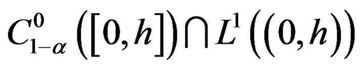
in the space .
.
Define

Clearly, it is closed, convex and nonempty.
Step I. We shall prove that we note that 
We note that

Since  it will be sufficient to impose

In view of the assumption  the second estimate is satisfied if say
  and
and  is chosen sufficiently small.
Step II. We shall prove that the operator  is compact. To prove the compactness of

defined by (5), it will be sufficient to argue on the operator
defined in this way:
We have  where the operator

Turn out to be compact from classical sufficient conditions, since . By Lemma 1.5, we have that Problem (3) has least a solution.
The proof is complete.
Lemma 1.7 Suppose that  satisfies H1,
 and
and  If
If  for some
  then the problem
 (6)
(6)
exists a positive constant  such that

Lemma 1.8 Let  with
with  Suppose further that
 . Then Problem (6) and its associated integral equation
 (7)
(7)
are equivalent.
Lemma 1.9 Assume that 
 satisfies H2, and
  for some
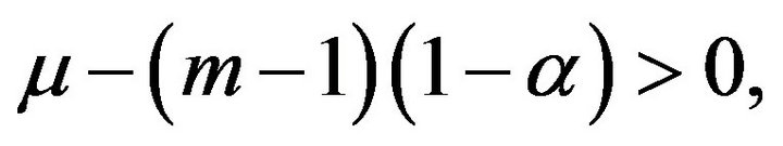
  Suppose further that
  then there exists
  and
and  such that any solution of (6) exists globally and satisfies
 (8)
(8)
2. Main Results
Theorem 2.1 Let  then initial problem (*) has a solution
  where
where


for all  and sufficiently small
Proof. Given  with eigenvalues
  by Lemma 1.3, there is a unitary matrix
  such that

is upper triangular with diagonal entries 
Let  we have

At the same time, the initial problem (*) changed into
 (**)
(**)
Now, let’s consider the problem (**).
Clearly, the problem (**) is equivalent to the following n problems

for  where
where  is the
  th entries of the vector
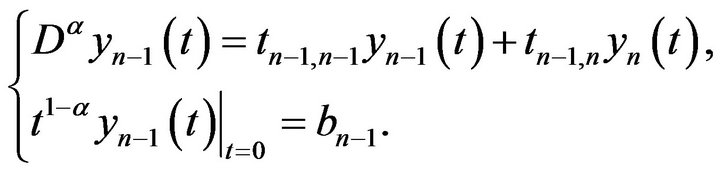
Consider the weighed Cauchy-type problem
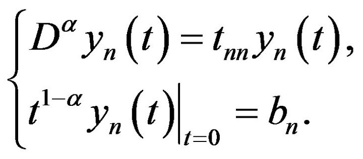
In Lemma 1.6, take  Then by lemma 1.6,
  s.t. the above problem has at least a solution

Consider the following weighed Cauchy-type problem

In Lemma 1.6, take  Then by Lemma 1.6,
  s.t. the above problem has at least a solution
Similarly, there has at least a solution in
for the rest n-2 initial problem in (**), denote by  respectively. And therefore, there has at least a solution

of the problem (**). Let 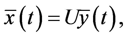 it is required for us.
The proof is completed.
Since the problem (**) is equivalent to the following n problems
 (9)
(9)
for  where
where  is the
  th entries of the vector
  Next, we shall discuss these equations in (9).
Theorem 2.2 Assume that the right hand of these equations in (9) satisfied H1, 
 and
and  for some
  If the solution of the problems (**) denoted by
 then there exists some constant
  such that
 for all
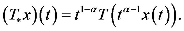
Proof. Similar to the proof of Theorem 2.1, now consider the following weighted Cauchy-type problem

Then by Lemma 1.7, there exists some constant  such that
Consider the following problem
Then by Lemma 1.7, there exists some constant  such that
Similarly, there exist some positive constants  such that

for all 
Let  Then we have
 for all
The proof is completed.
Theorem 2.3 Assume that  the right-hand of these equations in (9) satisfied H2, and
For some  Suppose further that

If denote solution of the problems (**) by
by

Then there exists some constant  and
and , such that

for all 
Using Lemmas 1.3 and 1.9, the proof is similar to Theorem 2.2. Therefore, it is omitted.
3. Acknowledgements
This research was supported by the NNSF of China (10961020), the Science Foundation of Qinghai Province of China (2012-Z-910) and the University Natural Science Research Develop Foundation of Shanxi Province of China (20111021).
NOTES