Forced Oscillation of Nonlinear Impulsive Hyperbolic Partial Differential Equation with Several Delays ()
1. Introduction
The theory of partial functional differential equations can be applied to many fields, such as biology, population growth, engineering, control theory, physics and chemistry, see the monograph [1] for basic theory and applications. The oscillation of partial functional differential equations has been studied by many authors see, for example [2] - [7] , and the references cited therein.
The theory of impulsive partial differential systems makes its beginning with the paper [8] in 1991. In recent years, the investigation of oscillations of impulsive partial differential systems has attracted more and more attention in the literature see, for example [9] - [13] . Recently, the investigation on the oscillations of impulsive partial differential systems with delays can be found in [14] - [19] .
To the best of our knowledge, there is little work reported on the oscillation of second order impulsive partial functional differential equation with delays. Motivated by this observation, in this paper we study the oscillation of nonlinear forced impulsive hyperbolic partial differential equation with several delays of the form
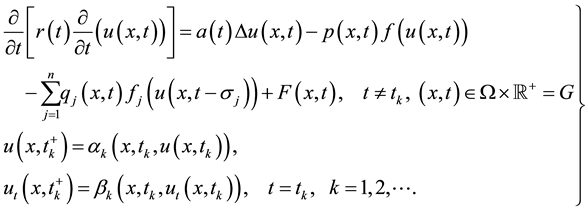 (1)
(1)
with the boundary conditions
 (2)
(2)
 (3)
(3)
and the initial condition
 (4)
(4)
Here  is a bounded domain with boundary
  smooth enough and
  is the Laplacian in the
Euclidean N-space ,
,  is a unit exterior normal vector of
 ,
,  ,
, 
In the sequal, we assume that the following conditions are fulfilled:
(H1) ,
,  is a positive constant,
  are class of functions which are
piece wise continuous in t with discontinuities of first kind only at ![]() and left continuous at
and left continuous at ![]()
(H2)![]() ;
; ![]() is a positive constant,
is a positive constant, ![]() is a positive constant, for
is a positive constant, for![]()
![]()
![]()
![]() and
and ![]()
![]()
(H3) ![]() and their derivatives
and their derivatives ![]() are piecewise continuous in t with discontinuities of first kind only at
are piecewise continuous in t with discontinuities of first kind only at ![]() and left continuous at
and left continuous at ![]()
![]()
![]()
![]()
(H4) ![]()
![]() and there exist positive constants
and there exist positive constants ![]() and
and ![]() such that for
such that for ![]()
![]()
![]()
Let us construct the sequence ![]() where
where ![]() and
and ![]()
![]()
By a solution of problem (1), (2) ((1),(3)) with initial condition (4), we mean that any function![]() for which the following conditions are valid:
for which the following conditions are valid:
1. If ![]() then
then ![]()
2. If ![]() then
then ![]() coincides with the solution of the problem (1) and (2) ((3)) with initial condition.
coincides with the solution of the problem (1) and (2) ((3)) with initial condition.
3. If![]() , then
, then ![]() coincides with the solution of the problem (1) and (2) ((3)).
coincides with the solution of the problem (1) and (2) ((3)).
4. If![]() , then
, then ![]() coincides with the solution of the problem (2) ((3)) and the following equations
coincides with the solution of the problem (2) ((3)) and the following equations
![]()
![]()
or
![]()
Here the number ![]() is determined by the equality
is determined by the equality ![]()
We introduce the notations:
![]()
![]()
![]()
The solution ![]() of problem (1), (2) ((1),(3)) is called nonoscillatory in the domain G if it is either eventually positive or eventually negative. Otherwise, it is called oscillatory.
of problem (1), (2) ((1),(3)) is called nonoscillatory in the domain G if it is either eventually positive or eventually negative. Otherwise, it is called oscillatory.
This paper is organized as follows: Section 2, deals with the oscillatory properties of solutions for the problem (1) and (2). In Section 3, we discuss the oscillatory properties of solutions for the problem (1) and (3). Section 4 presents some examples to illustrate the main results.
2. Oscillation Properties of the Problem (1) and (2)
To prove the main result, we need the following lemmas.
Lemma 2.1. Suppose that ![]() is the minimum positive eigenvalue of the problem
is the minimum positive eigenvalue of the problem
![]()
![]()
and ![]() is the corresponding eigenfunction of
is the corresponding eigenfunction of![]() . Then
. Then ![]() and
and ![]() Proof. The proof of the lemma can be found in [20] .
Proof. The proof of the lemma can be found in [20] . ![]()
Lemma 2.2. Let ![]() be a positive solution of the problem (1), (2) in G. Then the functions
be a positive solution of the problem (1), (2) in G. Then the functions
![]()
are satisfies the impulsive differential inequality
![]() (5)
(5)
![]() (6)
(6)
![]() (7)
(7)
where
![]()
has an eventually positive solution.
Proof. Let ![]() be a positive solution of the problem (1), (2) in G. Without loss of generality, we may assume that there exists a
be a positive solution of the problem (1), (2) in G. Without loss of generality, we may assume that there exists a ![]() such that
such that ![]() for
for
![]()
For ![]() multiplying Equation (1) with
multiplying Equation (1) with![]() , which is the same as that in Lemma 2.1 and then integrating (1) with respect to x over
, which is the same as that in Lemma 2.1 and then integrating (1) with respect to x over ![]() yields
yields
![]()
By Green’s formula, and the boundary condition we have
![]()
where ![]() is the surface element on
is the surface element on![]() .
.
Also from condition (H2), and Jenson’s inequality we can easily obtain
![]()
![]()
Thus, ![]() Hence we obtain the following differential inequality
Hence we obtain the following differential inequality
![]()
![]()
where
![]()
For ![]() from (1) and condition (H4), we obtain
from (1) and condition (H4), we obtain
![]()
![]()
According to ![]() we obtain
we obtain
![]()
![]()
Hence, we obtain that ![]() is a positive solution of impulsive differential inequalities (5)-(7).
is a positive solution of impulsive differential inequalities (5)-(7).
This completes the proof. ![]()
Lemma 2.3. Let ![]() be a positive solution of the problem (1), (2) in G. If we further assume that
be a positive solution of the problem (1), (2) in G. If we further assume that ![]()
![]() and the impulsive differential inequality (5), and
and the impulsive differential inequality (5), and
![]() (8)
(8)
![]() (9)
(9)
![]() (10)
(10)
have no eventually positive solution, then each nonzero solution of the problem (1)-(2) is oscillatory in the domain G.
Proof. Let ![]() be a positive solution of the problem (1), (2) in G. Without loss of generality, we may assume that there exists a
be a positive solution of the problem (1), (2) in G. Without loss of generality, we may assume that there exists a ![]() such that
such that![]() , for
, for ![]()
From Lemma 2.2, it follows that the function ![]() is an eventually positive solution of the inequality (5) which is a contradictions.
is an eventually positive solution of the inequality (5) which is a contradictions.
If ![]() for
for ![]() then the function
then the function
![]()
is a positive solution of the following impulsive hyperbolic equation
![]()
![]()
![]()
![]()
and satisfies
![]()
![]()
where
![]()
For ![]() from (1) and condition (H4), we obtain
from (1) and condition (H4), we obtain
![]()
![]()
According to ![]() we obtain
we obtain
![]()
![]()
Thus, it follows that the function ![]() is a positive solution of the inequality (8)-(10) for
is a positive solution of the inequality (8)-(10) for![]() which is also a contradiction. This completes the proof.
which is also a contradiction. This completes the proof. ![]()
Now, if we set ![]() in the proof of Lemma 2.3, then we can obtain the following lemma.
in the proof of Lemma 2.3, then we can obtain the following lemma.
Lemma 2.4. Let ![]() be a positive solution of the problem (1), (2) in G. If we further assume that
be a positive solution of the problem (1), (2) in G. If we further assume that ![]()
![]() and the impulsive differential inequality (5), and
and the impulsive differential inequality (5), and
![]() (11)
(11)
![]() (12)
(12)
![]() (13)
(13)
has no eventually positive solution, then each nonzero solution of the problem (1), satisfying the boundary condition
![]()
is oscillatory in the domain G.
Proof. Let ![]() be a positive solution of the problem (1), (2) in G. Without loss of generality, we may assume that there exists a
be a positive solution of the problem (1), (2) in G. Without loss of generality, we may assume that there exists a ![]() such that
such that ![]() for
for
![]()
From Lemma 2.2, it follows that the function ![]() is an eventually positive solution of the inequality (5) which is a contradiction.
is an eventually positive solution of the inequality (5) which is a contradiction.
If ![]() for
for ![]() then the function
then the function ![]() is a positive solution of the following impulsive hyperbolic equation
is a positive solution of the following impulsive hyperbolic equation
![]()
![]()
![]()
![]()
and satisfies
![]()
![]()
For ![]() from (1) and condition (H4), we obtain
from (1) and condition (H4), we obtain
![]()
![]()
According to ![]() we obtain
we obtain
![]()
![]()
Thus it follows that the function ![]() is a positive solution of the inequality (11)-(13) for
is a positive solution of the inequality (11)-(13) for ![]() which is also a contradiction. This completes the proof.
which is also a contradiction. This completes the proof. ![]()
Lemma 2.5. Assume that
(A1) the sequence ![]() satisfies
satisfies ![]()
![]() ;
;
(A2) ![]() is left continuous at
is left continuous at ![]() for
for ![]()
(A3) for ![]() and
and ![]()
![]()
![]()
where![]() ,
, ![]() and
and ![]() are constants. PC denote the class of piecewise continuous function from
are constants. PC denote the class of piecewise continuous function from ![]() to
to![]() , with discontinuities of the first kind only at
, with discontinuities of the first kind only at ![]()
Then
![]()
Proof. The proof of the lemma can be found in [21] . ![]()
Lemma 2.6. Let ![]() be an eventually positive (negative) solution of the differential inequality (11)-(13).
be an eventually positive (negative) solution of the differential inequality (11)-(13).
Assume that there exists ![]() such that
such that ![]()
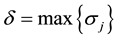
![]() for
for ![]() If
If
![]() (14)
(14)
hold, then ![]()
![]() for
for ![]() where
where ![]()
Proof. The proof of the lemma can be found in [22] . ![]()
We begin with the following theorem.
Theorem 2.1. If condition (14), and the following condition
![]() (15)
(15)
hold, where
![]()
then every solution of the problem (1), (2) oscillates in G.
Proof. Let ![]() be a nonoscillatory solution of (1), (2). Without loss of generality, we can assume that there exists
be a nonoscillatory solution of (1), (2). Without loss of generality, we can assume that there exists ![]() such that
such that ![]()
![]()
![]() for
for ![]()
From Lemma 2.4, we know that ![]() is a positive solution of (11)-(13). Thus from Lemma 2.6, we can find that
is a positive solution of (11)-(13). Thus from Lemma 2.6, we can find that ![]() for
for ![]()
For ![]()
![]()
![]() define
define
![]()
Then we have ![]()
![]()
![]() We may assume that
We may assume that ![]() thus we have that for
thus we have that for ![]()
![]() (16)
(16)
![]() (17)
(17)
![]() (18)
(18)
Substitute (16)-(18) into (11) and then we obtain,
![]()
Hence we have
![]()
or
![]()
From above inequality and condition ![]() it is easy to see that the function
it is easy to see that the function ![]() is nonincreasing for
is nonincreasing for![]() Thus
Thus ![]() for
for ![]() which implies that
which implies that
![]()
From (12)-(13), we obtain
![]()
and
![]()
![]()
Let
![]()
Then according to Lemma 2.5, we have
![]()
Since ![]() the last inequality contradicts condition (15). This completes the proof.
the last inequality contradicts condition (15). This completes the proof. ![]()
3. Oscillation Properties of the Problem (1) and (3)
Next we consider the problem (1) and (3). To prove our main result we need the following lemmas.
Lemma 3.1. Suppose that ![]() is the smallest positive eigen value of the problem
is the smallest positive eigen value of the problem
![]()
and ![]() is the corresponding eigen function of
is the corresponding eigen function of![]() . Then
. Then ![]() and
and ![]()
Proof. The proof of the lemma can be found in [20] . ![]()
Lemma 3.2. Let ![]() be a positive solution of the problem (1), (3) in G. Then the function
be a positive solution of the problem (1), (3) in G. Then the function
![]()
are satisfies the impulsive differential inequality
![]() (19)
(19)
![]() (20)
(20)
![]() (21)
(21)
where
![]()
has the eventually positive solution
![]()
Proof. Let ![]() be a positive solution of the problem (1), (3) in G. Without loss of generality, we may assume that there exists a
be a positive solution of the problem (1), (3) in G. Without loss of generality, we may assume that there exists a ![]() such that
such that ![]() for
for
![]()
For ![]() multiplying equation (1) with
multiplying equation (1) with![]() , which is the same as that in
, which is the same as that in
Lemma 3.1 and then integrating (1) with respect to x over ![]() yields
yields
![]()
By Green’s formula, and the boundary condition we have
![]()
where ![]() is the surface element on
is the surface element on![]() .
.
From condition (H2), we can easily obtain
![]()
![]()
The proof is similar to that of Lemma 2.1 and therefore the details are omitted. ![]()
Lemma 3.3. Let ![]() be a positive solution of the problem (1), (3) in G. If we further assume that
be a positive solution of the problem (1), (3) in G. If we further assume that ![]()
![]() and the impulsive differential inequality (19), and
and the impulsive differential inequality (19), and
![]() (22)
(22)
![]() (23)
(23)
![]() (24)
(24)
have no eventually positive solution, then each nonzero solution of the problem (1), (3) is oscillatory in the domain G.
Proof. The proof is similar to Lemma 2.3, and hence the details are omitted. ![]()
Futhermore, if we set![]() , then we have the following lemma.
, then we have the following lemma.
Lemma 3.4. Let ![]() be a positive solution of the problem (1), (3) in G. If we further assume that
be a positive solution of the problem (1), (3) in G. If we further assume that ![]()
![]() and the impulsive differential inequality (19), and
and the impulsive differential inequality (19), and
![]() (25)
(25)
![]() (26)
(26)
![]() (27)
(27)
has no eventually positive solution, then each nonzero solution of the problem (1), satisfying the boundary condition
![]()
is oscillatory in the domain G.
Proof. The proof is similar to Lemma 2.4, and hence the details are omitted. ![]()
Using the above lemmas, we prove the following oscillation result.
Theorem 3.1. If condition (14) and the following condition
![]() (28)
(28)
hold, where
![]()
then every solution of the problem (1), (3) oscillates in G.
Proof. Let ![]() be a nonoscillatory solution of (1), (3). Without loss of generality, we can assume that there exists
be a nonoscillatory solution of (1), (3). Without loss of generality, we can assume that there exists ![]() such that
such that ![]()
![]()
![]() for
for ![]()
From Lemma 3.4, we know that ![]() is a positive solution of (25)-(27). Thus from Lemma 2.6, we can find that
is a positive solution of (25)-(27). Thus from Lemma 2.6, we can find that ![]() for
for ![]()
For ![]()
![]()
![]() define
define
![]()
Then we have ![]()
![]()
![]() We may assume that
We may assume that ![]() thus we have that for
thus we have that for ![]()
![]() (29)
(29)
![]() (30)
(30)
![]() (31)
(31)
We substitute (29)-(31) into (25) and can obtain the following inequality,
![]()
then we have
![]()
From (26)-(27), we can obtain
![]()
It follows that
![]()
![]()
Let
![]()
Then according to Lemma 2.5, we have
![]()
Since ![]() the last inequality contradicts (28). This completes the proof.
the last inequality contradicts (28). This completes the proof. ![]()
Theorem 3.2. If condition (14) and the following condition
![]() (32)
(32)
hold for some![]() , then every solution of the problem (1), (3) oscillates in G.
, then every solution of the problem (1), (3) oscillates in G.
Proof. The proof is obvious and hence the details are omitted. ![]()
4. Examples
In this section, we present some examples to illustrate the main results.
Example 4.1. Consider the impulsive differential equation
![]() (33)
(33)
and the boundary condition
![]() (34)
(34)
Here ![]()
![]()
![]() and taking
and taking ![]()
Moreover
![]()
so (14) holds. We take![]() , then
, then
![]()
thus
![]()
Hence (28) holds. Therefore all conditions of Theorem 3.1 are satisfied. Hence every solution of the problem (33), (34) oscillates in ![]() In fact
In fact ![]() is one such solution of the problem (33) and (34).
is one such solution of the problem (33) and (34).
Example 4.2. Consider the impulsive differential equation
![]() (35)
(35)
and the boundary condition
![]() (36)
(36)
Here ![]()
![]()
![]()
![]()
![]()
![]()
![]()
![]()
![]()
![]()
![]() and taking
and taking
![]() It is easy to check that the conditions of Theorem 2.1 are satisfied. Therefore, every solution
It is easy to check that the conditions of Theorem 2.1 are satisfied. Therefore, every solution
of the problem (35), (36) oscillates in ![]() In fact
In fact ![]() is one such solution of the problem (35) and (36).
is one such solution of the problem (35) and (36).
Acknowledgements
The authors thank Prof. E. Thandapani for his support to complete the paper. Also the authors express their sincere thanks to the referee for valuable suggestions.