Simulation on Cavitation Bubble Collapsing with Lattice Boltzmann Method ()
1. Introduction
Ultrasonic cavitation is applied extensively in industry and agriculture production. Since 1960s, people understood the cavitation effect, cleaning, underwater cutting, sewage treatment, ultrasonic cleaning, oil drilling and other operations. Cavitation damage to solid surface is a major concern on the design of turbo―machinery and there have been many investigations on the bubble behavior or bubble dynamics near solid wall [1]. The causes and mechanism of cavitation bubble collapse near solid wall are still not perfect, and the exploration of these problems will be the cavitation effect to step into industrial production and make a good foundation in engineering application.
The lattice Boltzmann method (LBM), as a novel mesoscopic [2] numerical algorithm, has attracted considerable attention over last decade. It is based on molecular dynamics and statistical mechanics, using simple rules of particle movement to approximate molecular mass, which can get the macroscopic fluid movement. LB equation (LBE) evolved from the lattice gas automatic (LGA), and introducing a probability distribution to reduce the statistical noise in calculating the LGA, which is an artificial microscopic model for gases, and it was shown that LBE could also be derived from the Boltzmann equation following some standard discretization later [3]. Due to the high dimension of the particle distribution function with a complex collision term continuous, Boltzmann equation for theoretical analysis and numerical method is challenging by direct solution. LBM is a method which is quite different from the traditional computational fluid dynamics (CFD) algorithms. From the physical essence, the kinetic behavior of multiphase flow system is the result of the microscopic interaction among fluid phase. Based on the theory of molecular motion, LBM is especially suitable for describe the complex multiphase flow from the underlying [4]. Meanwhile, the CFD method such as volume of fluid (VOF) [5] level set method (LSM) [6], how to consider the pressure and interaction between electromagnetic field and capillary effect in the multiphase flow calculation has been a challenge all the time. For the flow of the surface tension, the VOF and LSM are unstable near the interface of numeric. Therefore, as a powerful tool for the numerical simulations and investigation of multiphase flows, the LBM has multiple advantages including time and space efficient computations that are straightforward to parallelize, handles complex boundaries without difficulty, and directly link between microscope and macroscopic phenomenon.
In recent years, pseudopotential Shan-Chen model is introduced into cavitation study frequently. The Shan- Chen model, which introduced inter-particle potential to describe the interactions among different phases or components, is the most widely used due to its simplicity, high computational efficiency and high flexibility [7]. Sukop and Or firstly followed the acoustic cavitation problems using the LBM Shan-Chen model [8]. Zhang Xinming investigated the 3 dimension (3D) cavitation bubble phenomenon on the low liquid pressure and successfully reproduced the bubbles growth in low pressure water [9]. Mishra [10] coupling between the hydrodynamics of a collapsing cavity and supported solute chemical species introduced of cavitation based on the Shan- Chen multiphase model. Chen [11] simulated the cavitating bubble growth with the modified Shan-Chen model with large density ratio in both quiescent and shear flows and compared with the Rayleigh-Plesset equation. Zhou and Shan [12] simulated the acoustic cavitation of spherical bubble and compared with the predictions of Keller equation to original Shan-Chen pseudopotential model. Recently, Shan and his group used modified Shan-Chen model found the second collapse in the rigid boundary damage of cavitation bubble and the impeding effect between two collapses successfully [13]. However, it should be mentioned that the report about cavitation bubble in square flume solid boundaries by LBM numerical simulation are fewer.
In this paper, the cavitation phenomenon based on a modified Shan-Chen model to simulate the collapse phase of bubble near the solid wall in square flume. The model is characterized by coupling with the Carnahan- Starling equation of state (C-S EOS) and the exact difference method (EDM) in the forcing term treatment.
2. Numerical Model and Simulation
2.1. Lattice Boltzmann Model
LBM have been proven to be efficient simulation tools for a variety of complex flow problems. It is based on the numerical simulation of a time-space and velocity-discrete Boltzmann-type equation. The LBM consists of two steps according to its theory: Step 1 is the streaming, where each particle moves to the nearest node along the direction of its velocity. Step 2 is the collision which occurs when several particles arrive at a node together and they interact and possibly charge their velocity directions in terms of the scattering rules. By the single relaxation time (SRT) Bhatnagar-Gross-Krook (BGK) approximation, these two steps can be combined into the following lattice Boltzmann Bhatnagar-Gross-Krook equation with a source term
 (1)
(1)
where  is the single-particle density distribution function related to the discrete velocity direction,
  is the Maxwell-Boltzmann distribution function,
  is the dimensionless relaxation time that is re-
lated to the kinematic viscosity by , this choice for the viscosity makes formally the LBGK scheme a second order method for incompressible flows [13]. Equation (1), termed the LBE [14] with BGK approximation or LBGK model, is usually solved in the following two steps:
Collision step:
 (2a)
(2a)
Streaming step:
 (2b)
(2b)
where  represents the post-collision state.
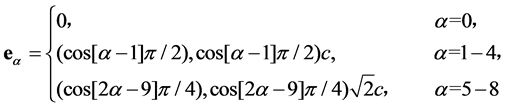
A particular two-dimensional LBGK model considered in this work is the nine velocity direction at a given point in two dimensional space model (D2Q9) [15]. In this model, discrete velocities are namely
 (3)
(3)
where  is a ratio,
  and
and  are the lattice space and the time step (time), respectively. From now on we shall use the units of
  and
and , and one mass unit as
  [16], such that all the relevant quantities are dimensionless. In the D2Q9 model (Figure 1), the equilibrium function is of the form
 (4)
(4)
where u is the fluid velocity,  is the weighting factor given by
![]() . (5)
. (5)
In the discretized velocity space, the density and momentum fluxes can be evaluated as
![]() (6)
(6)
and
![]() (7)
(7)
The speed of sound in this model is![]() .
.
We choose to work on single component multiphase fluids an attractive force ![]() between nearest neighbor fluid particles is need, for the D2Q9 model, we have
between nearest neighbor fluid particles is need, for the D2Q9 model, we have
![]() (8)
(8)
where ![]() is the interaction strength,
is the interaction strength, ![]() is given by
is given by
![]() (9)
(9)
And ![]() is an interaction potential
is an interaction potential
![]() (10)
(10)
where ![]() and
and ![]() are arbitrary constants, the interaction potential function
are arbitrary constants, the interaction potential function ![]() must be monotonically increasing and bounded [17]. Application of Equation (6) and (7) leads to a non-ideal equation of state (EOS)
must be monotonically increasing and bounded [17]. Application of Equation (6) and (7) leads to a non-ideal equation of state (EOS)
![]() (11)
(11)
where![]() . Equation (11) is a nonmonotonic increasing function at a single pressure, and has the essential feature of the vander Waals EOS (vdW EOS) that allows liquid-vapor phase coexistence. When the value of G is less than the critical value of interaction strength
. Equation (11) is a nonmonotonic increasing function at a single pressure, and has the essential feature of the vander Waals EOS (vdW EOS) that allows liquid-vapor phase coexistence. When the value of G is less than the critical value of interaction strength![]() , phase separation will occurs.
, phase separation will occurs.
Using the method developed by [18], Equation (11) can be expressed by
![]() (12)
(12)
where ![]() is the lattice sound speed. With this method, different EOS can be substituted into Equation (12). Modified with the vdW EOS, we can obtain C-S EOS
is the lattice sound speed. With this method, different EOS can be substituted into Equation (12). Modified with the vdW EOS, we can obtain C-S EOS
![]() (13)
(13)
where![]() ,
,![]() . Here
. Here ![]() and
and ![]() are the critical temperature and pressure, respectively [16].
are the critical temperature and pressure, respectively [16].
In Reference [19] [20], the force term in the Equation (1) can be expression as
![]() (14)
(14)
where F is the total force acting on a fluid particle, which contains all possible external forces.
2.2. Computational Domain and Parameter Setting
For the cavitation bubble near solid walls, the computational domain consists of 401 × 401 grid nodes for bubble collapse simulation as shown in Figure 2, the adhesion between fluid and solid wall is setting as zero. The bubble is therefore taken to be spherical and gravity is also omitted. Vapor pressure is uniform throughout the bubble interior. The equilibrium phase density are obtains vapor pressure and liquid pressure. Simulating a series of different initial radius of bubble equilibrium state of pressure difference inside and outside surface tension can be obtained. In addition, if it is not specially announced, the lattice unit is adopted for all data. The initial radius of bubble is R0 = 60.
The present choice of parameters a, R, b in the CS EOS![]() ,
, ![]() ,
, ![]() is appropriate [16]. The analytical densities at a specified temperature and zero velocity are used as initial conditions. The density field is initialized as
is appropriate [16]. The analytical densities at a specified temperature and zero velocity are used as initial conditions. The density field is initialized as
![]() (15)
(15)
where![]() ,
, ![]() is the center position of the bubble, and the hyperbolic tangent function is
is the center position of the bubble, and the hyperbolic tangent function is![]() ,
, ![]() , is a width of the phase interface. And the parameters of critical value and dimensionless value are given in Table 1, Table 2, respectively.
, is a width of the phase interface. And the parameters of critical value and dimensionless value are given in Table 1, Table 2, respectively.
![]()
Figure 2. Physical model (R0―bubble initial radius; b―distance between the bubble centre and solid wall;![]() ―vapor pressure in bubble;
―vapor pressure in bubble;![]() ― ambient pressure).
― ambient pressure).
![]()
Table 1. The critical value of T, P, ρ.
![]()
Table 2. The dimensionless value and lattice value of T, ρ.
2.3. Boundary Condition
The bubble is located in the center of square flume, the distance equidistant from right and left rigid wall. Zou- He pressure boundary conditions were applied in top, left and right directions. Meanwhile, we adopted standard bounce-back format in the bottom wall [17] [21] [22].
3. Results and Discussion
3.1. Bubble Form
The bubble profiles evolution was introduced detailed, which can refer to [23] [24]. From the Figure 3 of density field, the same physical value parameters of computational domain simulated between experiment [23] results and LBM. Due to the pressure of the top boundary, which the collapse phase the bubble migrates strongly towards the bottom wall being under equal influence of the left and right solid wall, and the result of LBM agree qualitatively with the previous experimental conclusion.
Simulation collapses of cavitation bubble in 2D pressure field in special time are shown in Figure 4. At the beginning the bubble is a standard spherical form (Figure 4(a)), at the top of the pressure with the migration of time step with the left and right solid wall, there are low pressure area near a solid wall, at the bottom of the bubble is effected of low pressure slightly compressed which is around the left, right and bottom walls (Figure 4(b)), bubble is no longer a spherical bubble. As the pressure migration, bubble compressed from the top of the conical high pressure region (Figure 4(c) and Figure 4(d)), the walls of the low pressure melted for high pressure from above, high pressure region appeared above the bubble. Meanwhile, bubble was compressed crosswise. Due to the effect of the constraint by the rigid wall, the pressure field of pull the bubble transverse is bigger than the pressure of rebound lengthways. With the approaching of the pressure above and aggravate, top and bottom wall of bubble was adhesion each other gradually (Figure 4(e)), bubble was collapsed into two sectional by pressure field, and the middle of bubble have been a high velocity jet. Cavitation bubble collapse near a solid wall developed a great deal of pressure difference, it was based on the original center of the circle of a low pressure ring, the pressure difference is the cause of the shock wave formed. Two bubbles are compressed until the positive pressure to crush (Figure 4(f)), this time as a result of the vapor pressure existing inside the bubble, the cavitation bubble will have second collapse phenomenon (Figure 4(g)). After the second collapse, negative and positive pressure rebound and expand gradually (Figures 4(h)-(j)), mixture pressure oscillate around in the area of the square overall until the two pressure fusion mutual.
3.2. Collapse Time
A solution for a particular value of ![]() can be scaled to bubble of any initial size under any positive collapsing pressure
can be scaled to bubble of any initial size under any positive collapsing pressure ![]() [25], Figure 5 provides details of the simulation results, With the increasing of pressure (pressure difference)/initial size, bubble collapse time diminishing. As shown in Figure 5(a),
[25], Figure 5 provides details of the simulation results, With the increasing of pressure (pressure difference)/initial size, bubble collapse time diminishing. As shown in Figure 5(a), ![]() is 0.0096 - 0.0165, change rate of collapse time fading quickly. When the pressure beyond 0.00165, collapse time
is 0.0096 - 0.0165, change rate of collapse time fading quickly. When the pressure beyond 0.00165, collapse time
drifts to a stable value. We can find that the initially spherical bubble starts to collapse due to the pressure difference between outside and inside of the bubble. As shown in Figure 5(b), ![]() is 1.2 - 2.0, collapse time change quickly. when
is 1.2 - 2.0, collapse time change quickly. when ![]() is beyond 2.0, the collapse time changes to be steady. In our simulation,
is beyond 2.0, the collapse time changes to be steady. In our simulation, ![]() more
more
than 2.0, in other words, the distance between bubble centre and solid wall which is twice the bubble initial radius, bubble just has one collapse. As shown in Figure 6, when ![]() is 1.2 - 2, the certain value of collapse time has founded.
is 1.2 - 2, the certain value of collapse time has founded.
3.3. Second Collapse
In order to understand the process of second collapse easily, Figure 7 shows the evolution of pressure field. As shown in Figure 7, the distance between bubble center and solid wall increases as λ gets bigger. In Figure 7(a), λ = 1.2, a1 and a2 are the first and second collapse in low pressure (LP,![]() ), respectively, while, in the same λ, a3 and a4 are the first and second collapse in high pressure(HP,
), respectively, while, in the same λ, a3 and a4 are the first and second collapse in high pressure(HP,![]() ), respectively. Cavitation is a transient complex phenomenon, during the collapse phase the bubble migrate and then develop a jet towards the closest bottom wall. Bubble collapse in high pressure is more violent than that in low pressure. High pressure gradient results in the more serious bubble deformation in Figure 7(a3) than the bubble deformation in Figure 7(a1), and much more violent bright bubble collapse in Figure 7(a4) than bubble collapse in Figure 7(a2). We can obtained the interval time of first and second collapse visual.
), respectively. Cavitation is a transient complex phenomenon, during the collapse phase the bubble migrate and then develop a jet towards the closest bottom wall. Bubble collapse in high pressure is more violent than that in low pressure. High pressure gradient results in the more serious bubble deformation in Figure 7(a3) than the bubble deformation in Figure 7(a1), and much more violent bright bubble collapse in Figure 7(a4) than bubble collapse in Figure 7(a2). We can obtained the interval time of first and second collapse visual.
![]()
![]() (a) (b)
(a) (b)
Figure 5. (Color online) Collapse time (![]() ).
).
![]()
Figure 6. (Color online) Time interval of two collapse (![]() ).
).
![]() (a) (b) (c) (d)
(a) (b) (c) (d)
Figure 7. The process of first bubble collapse to secondary collapse in 2D pressure field.
4. Conclusion
In this paper, a new method based on modified Shan-Chen pseudo potential lattice Boltzmann method is used to simulation on cavitation bubble collapsing in 2D press filed. It is found that the method gives a visual physical prospect to investigation the 2D pressure filed evaluation and the collapse time of the cavitation bubble. The simulation results on the bubble shape are quantitatively in good agreement with experiment observation. However, these problems could be solved if acoustic pressure can be introduced into the model by setting the values of distribution function ![]() at top boundary [12], which we can solve the cavitation bubble in complex geometric boundary with acoustic field or dimensionless electromagnetic field [26]. Although this model has numerous shortcomings, this work demonstrates that investigation on cavitation bubble with LBM is very suitable and effective during the process of collapse between first and second collapse, and interval time was founded. Furthermore, the method has a widely use when the model modified in acoustic field.
at top boundary [12], which we can solve the cavitation bubble in complex geometric boundary with acoustic field or dimensionless electromagnetic field [26]. Although this model has numerous shortcomings, this work demonstrates that investigation on cavitation bubble with LBM is very suitable and effective during the process of collapse between first and second collapse, and interval time was founded. Furthermore, the method has a widely use when the model modified in acoustic field.
Acknowledgements
The author deeply appreciates the discussion with Dr. Minglei Shan. Project No.11174191 was supported by the National Science Foundation of China.
NOTES
*Corresponding author.