Adaptive Strategies for Accelerating the Convergence of Average Cost Markov Decision Processes Using a Moving Average Digital Filter ()
1. Introduction
Discrete-time Markov decision processes aim at controlling the dynamics of a stochastic system by mean of taking suitable control actions at each possible configuration of the system. At each period, a control action is selected based on the current configuration (state) of the system, which triggers a probabilistic transition to another state in the next decision period and so on in an infinite time horizon. The objective is to find the best action to be taken at each possible configuration of the system with respect to some prescribed performance measure. From now on, each configuration of the system is referred to as a state of the system.
An elegant way to find the optimal control actions for each state is provided by the classical value or policy iteration algorithms [1-11]. The value iteration (VI) algorithm is arguably the most popular algorithm, in part because of its simplicity and ease of implementation. In this paper, we introduce an adaptive way to improve the convergence of the VI algorithm with respect to convergence time, with a view at accelerating the convergence of the method. We refer to [12] for a study on variants of the policy iteration algorithm.
We explore a way to accelerate the convergence of value iteration algorithms for average cost MDPs. The rationale is to apply the value iteration algorithm to a sequence of approximate models, which are simpler than the original model and hence require less computation. These models are refined at each new iteration of the algorithm and converge to the exact model within a finite number of iterations, which enables one to retrieve the solution to the original problem at the end of the procedure. The rationale is based on a refinement scheme introduced in [13] for linearly convergent algorithms with convergence rates that are known a priori.
Classical Markov Decision Problem (MDP) results yield that VI algorithms converge, but the rate of convergence is unknown a priori and depends on the system at hand. For more details on the convergence of VI algorithms for average cost MDPs, we refer to [1]. The unknown rate of convergence renders the results in [13] not directly applicable for the studied problem. Earlier results, however, have shown that significant reduction on the overall computational effort can be attained by a suitable choice of refinement rate [14]. Unfortunately, such rate is now known a priori and the parameter tuning turns out to be very difficult. Moreover, consistent performance gains over the classical VI algorithm are difficult to obtain and a poor parameter selection may render the algorithm slower than classical VI. In this paper, we try to overcome this difficulty by introducing an adaptive algorithm that automatically adjusts the refinement rate at each iteration. It employs the error sequence of the algorithm to iteratively estimate the empirical convergence rate, and a moving average digital filter is appended to mitigate the erratic behavior. For more details about moving average filters, we refer to [15]. We show that the adaptive algorithm presents a robust performance, consistently outperforming value iteration.
2. Average Cost Markov Decision Processes
Markov decision processes are comprised of a set of states, each representing a possible configuration of the studied system. Let  be the set of all possible system configurations. For each state
 , there exists a set of possible control actions
 . Each action
  drives the system from state
  to state
  with probability
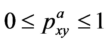 . Since
  is a probability for all
  and
and  in
in , we have
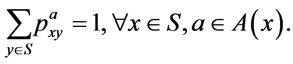
Let  be the set of all possible control actions and
  represent a cost function in the state/action space. When visiting state
  and applying a control action
 , the system incurs a cost
 . A stationary control policy is a mapping from the state space
  to the action space
  that defines a single action in
  to be taken each time the system visits state
 . Let
. Let  denote any particular stationary policy and
  denote the set of all feasible stationary control policy.
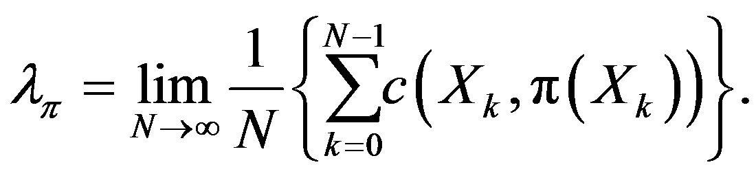
Once a stationary control policy  is chosen and applied, the controlled system can be modeled as a homogeneous Markov chain
  [16]. The long term cost of the system that operates under policy
  is given by
 (1)
(1)
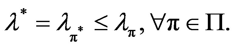
Under general conditions [1], each control policy  implies a finite long term cost
 . The task of the decision maker is to identify a policy
  that minimizes the long term average cost, thus satisfying the expression below:
 (2)
(2)
In order to find the optimal policy, one seeks for the solution to the Poisson Equation (Average Cost Optimality Equation):
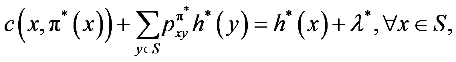 (3)
(3)
which is satisfied only by the optimal policy, where  is a real valued function, sometimes referred to as value function or relative cost function.
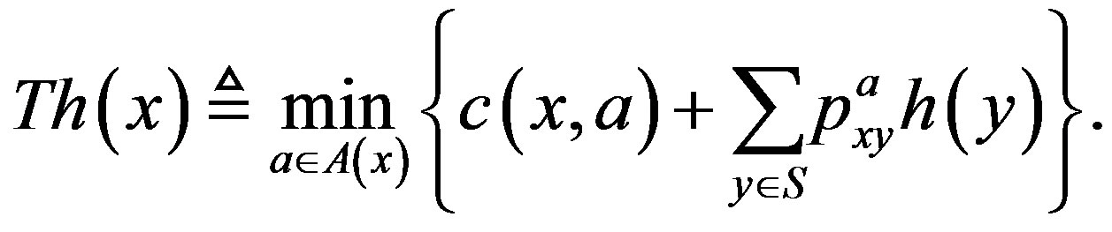
3. The Value Iteration Algorithm
A very popular algorithm to find the optimal policy  is the value iteration (VI) algorithm. This algorithm iteratively searches for the solution
  to the Poisson Equation (3).
Let  be the space of real valued functions in
 . The VI algorithm employs a mapping
  defined as
 (4)
(4)
The VI algorithm consists in applying the recursion
 (5)
(5)
to obtain increasingly refined estimates of the solution to the Poisson Equation (3). Under mild conditions [1], the algorithm can be shown to converge to the solution of Equation (3), thus yielding both the optimal policy  and its associated average cost
 .
.
The convergence of the algorithm is linear, but the rate of convergence is not known a priori [1].
4. The Partial Information Value Iteration Algorithm
The rationale behind the partial information value iteration (PIVI) algorithm is to iterate on increasingly refined approximate models that converge to the exact model according to a prescribed schedule defined a priori. The purpose of such a refinement is to employ less computational resources in the early states of the algorithm, when the algorithm is typically far from the optimal solution, and hence focus most of the computational resources within a region that is closer to the optimal solution.
An intuitive way of decreasing the computational effort at the early iterations is to focus on the most probable transitions at the initial stages of the algorithm. For any state-action pair  let
let 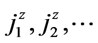 be an ordering of the states in decreasing order of transition probabilities, that is
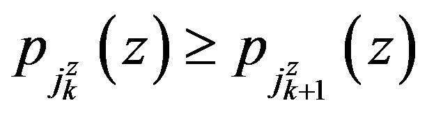 . This leads to the distribution functions
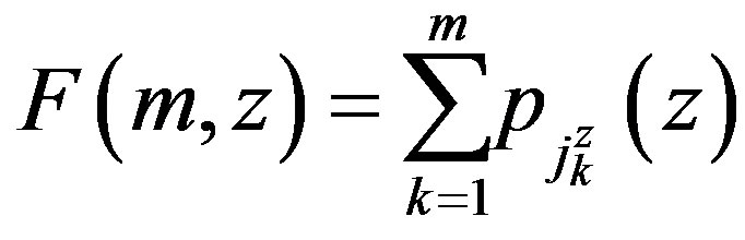
Let
 (6)
(6)
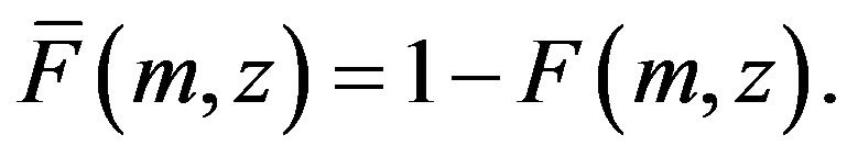
where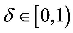 .
.
Consider the following mapping [13]
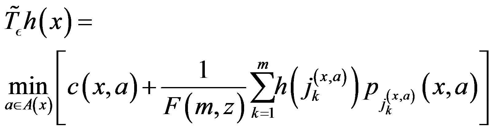 (7)
(7)
where 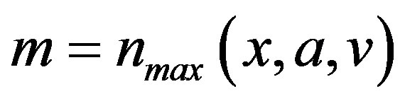 and
and  is a normalizing factor intended to make the truncated transition probability into a normalized probability distribution. Let
  be a limited non-increasing sequence in the interval
  such that
 (8)
(8)
The PIVI algorithm can be defined by the following recursion
 (9)
(9)
Observe that, since the parameter sequence  in (8) goes to zero, the algorithm tends to the exact algorithm and, as such, converges to the solution to the proposed problem. This follows by applying (5) to some iterate
  in (9), with an arbitrarily high index
  relabeled as zero.
4.1. The Parameter Sequence 
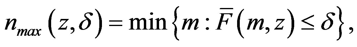
As pointed out in the last section, it suffices that  goes to zero within finite time for the PIVI algorithm (9) to converge to the exact solution. Hence, the sequence
  can be freely selected from the class of convergent sequences in the interval
  whose limit is nil. However, it is the form at which the convergent sequence goes to zero that will ultimately determine the behavior and, therefore, the computational effort, of the PIVI algorithm [13,14].
It has been shown that, for linearly convergent algorithms with convergence rate  the optimal sequence with respect to the overall computational effort is geometrically decreasing, with rate
 , which coincides with the convergence rate of the algorithm [13]. This result applies to discounted MDPs, for which the convergence rate
  is known and coincides with the discount factor.
Average cost MDPs do converge linearly, but the convergence rate is unknown and depends on the topology of the MDP being solved [1]. This renders the direct application of the results in [13] unpractical. Indeed, geometrically decreasing sequences  where tried in [14], and promising results where obtained. The difficulty in such an approach lies in the fact that guessing the convergent rate a priori can be quite a daunting task. Indeed, when a suitable decreasing rate is found, it can result in significant computational savings. However, a poor choice of decreasing may result in an inefficient algorithm, which can even be outperformed by standard value iteration [14]. In this paper we address this short-coming by introducing an algorithm that adaptively decreases the error sequence
 , and that results in a more robust algorithm, with more stable behavior that consistently outperforms standard value iteration.
4.2. Identification of Efficient Parameter Sequences
In this section we propose an adaptive algorithm to adaptively select the parameter sequence . The selection is based on the span semi-norm of the error sequence obtained by the PIVI algorithm at each iteration, defined as
 (10)
(10)
where  is the result of the k-th iterate of Algorithm (9).
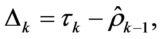
The proposed algorithm uses the error defined above to assess the empirical convergence rate at iteration ,
,  , defined as:
 (11)
(11)
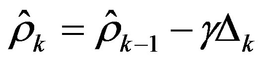
During the convergence process, the error  should steadily decay. It is possible, however, that the decrease in parameter
  in mapping
  in the PIVI algorithm (9), which is defined in (7), results in an immediate increase in the error. This happens because a decrease in
  results in a different, more accurate approximate model in (7), for which the current approximation in the value function
  may not be as good. Hence, in order to avoid instability, i.e., a
 , whenever the error increases,
  is set to zero.
For the adaptive algorithm, we use a varying decrease rate sequence  and the objective is to adaptively estimate the convergence rate of the exact algorithm, which is unknown a priori. In order to do that, gradient,
  is calculated, which is defined as:
 (12)
(12)
The convergence parameter is estimated by the adaptive gradient recursion Equation as follows:
 (13)
(13)
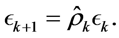
where , and
, and  is an adaptive parameter. The parameter sequence
  in Algorithm (9) is then refined by the following recursion:
 (14)
(14)
The proposed parameters sequence,  , may result in an intensely varying sequence
 , due to a possible erratic behavior in the error sequence
  and such a variation may limit the computational gains. To mitigate the effect of the error on the estimation process, a refined algorithm is presented. Prior to estimating the empirical convergence rate Equation (11), the error,
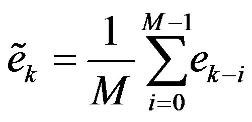
  , goes through moving average digital filter of order
  [15]. This filter attenuates the error high frequency components, leading to a better estimation of the convergence rate parameter,
 . The differences Equation that implements the moving average filter is presented in (15).
 (15)
(15)
where  is the filter input, and
  is the filtered error, and
  is the filter order. The filter uses
  past iterations to estimate the error
 . The estimated error is used in (11) to approximate the empirical convergence rate. The higher the filter order
 , the longer the past history that is taken into account.
4.3. A Measure for Computational Effort Comparison
In order to compare the overall computational effort, one needs to propose a measure of the total computational effort applied by each algorithm. Such a measure enables one to directly compare different types of algorithms, which can rely on different updating schemes. In addition, defining this type of measure is more appealing than just measuring the convergence time because it makes possible to compare different types of algorithms without necessarily running them. Furthermore, one can also define suitable optimization routines that aim at finding the best algorithm in a given class with respect to the overall computational effort. This line of study is exploited in [13].
Examining the updating scheme of mapping  in the VI algorithm (5), it can be verified that the overall computational effort per iteration, per state, of the VI algorithm is proportional to the total number of transitions examined by mapping
 . Hence, one can define the computational effort of updating a single state
  as the sum of the cardinalities of the transition probability distributions for each feasible action for that state. Let
  denote the computational effort of updating state
  under the VI algorithm. The overall effort for a single iteration of the VI algorithm then becomes
The computational effort for an iteration of the PIVI algorithm, on the other hand, depends on the total number of transitions examined in each iteration of the algorithm. Letting  denote the parameter sequence of the PIVI algorithm and
  denote the total number of transitions at state
 , at the k-th iteration of the PIVI algorithm, we have
 (16)
(16)
where  is the function defined in (6) for stateaction pairs
 . Let
. Let  denote the total number of iterations up to the PIVI convergence. Consequently, the overall computational effort of the PIVI algorithm becomes
In the next section, we experiment with the parameter sequence , varying the adaptive parameter
  in (13) and compare the computational effort measures
  and
and , to obtain the order of the computational savings that can be obtained by the PIVI algorithm when compared to the classical VI algorithm.
5. Numerical Experiments
In order to compare the proposed method with the classic VI algorithm [17], two sets of experiments were derived. These experiments are replications of the experiments presented in [14] and thus offer a ground for comparison. In the first experiment we solve a Queueing model with two classes of clients. Each client class has a dedicated queue whose length varies in the interval . Moreover, no new client is permitted at any given queue whenever the length of that queue is at the upper limit. For both experiments, a single server is responsible for the service of both queues and serves
  clients at each time period. The decision maker must decide whether to serve Queue 1, Queue 2, or to stay idle. The cost function depends on the total of clients in line and is given by:
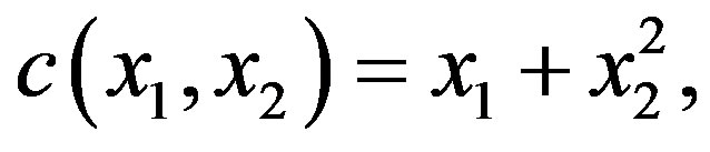
where  and
and  denotes the size of Queue 1 and Queue 2, respectively. Clearly, such a cost function is designed to prioritize clients belonging to the second class. We also note that the cost function does not depend on the selected control actions. The objective is to find the policy which minimizes the average cost and satisfies expression (2).
For the first experiment, both types of clients arrive according to a Poisson process with mean . For computational purposes, the transition probability generated by this process was truncated to accommodate a fraction 0.9999 of the transitions and re-normalized afterwards. Such a normalization yields a total of 22 transitions for each line, thus resulting in a total of 484 possible transitions for each state-action pair. For this experiment
  was fixed at 21. Since we have three possible control actions and since the number of transitions is the same under each action, the total number of transitions per state for the VI algorithm is
For a tolerance of  [1], the VI algorithm took 950 iterations to converge, having an overall computational effort per state of
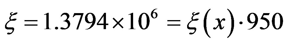 , per state. The total effort can be obtained by multiplying this value by the cardinality of the state space S,
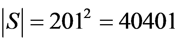 .
.
Figure 1 depicts the overall computational effort  for parameter sequences of the type in (14), for different values of
 . The computational effort was normalized with respect to the overall VI effort
  to simplify the comparison.
The normalized computational effort for the proposed algorithm is plotted in Figure 1 as a function of the adaptive parameter . One can see that, for the best
 (a)
(a) (b)
(b)
Figure 1. Computational effort: Poisson distribution. (a) filter orders M = 4, 5, 7, and 8; (b) filter orders M = 9, 10, and 11.
possible choice of , the computational effort is approximately
  of that of the classical VI algorithm. Therefore, the proposed algorithm converges in about
  of the time required for the VI algorithm to converge. Another point to look at is the improvement due to the moving average digital filter. Five curves are shown in Figure 1(a), the solid blue curve is the overall computational effort without filtering of the empirical rate; the square-marked dotted line curve, the circle-marked dashed line curve, the diamond-marked dashed line curve, and the triangle-marked solid line curve present the computational effort with the moving average digital filter defined in (15) of orders
 , respectively. This filters are used to process the error sequence
  prior to the empirical rate estimation in (11). While the unfiltered algorithm produces an improvement over the classic VI algorithm, the use the moving average filter provides an even superior performance, since the filter acts as a smoother of fluctuations in the empirical error function. Moreover, one can see that the performance improves as the filter order increases.
Figure 1 also shows that the proposed algorithm is consistently better than the VI algorithm, for a broad range of parameters . Naturally, a better choice of parameter results in better savings, but the results suggest that the algorithm is robust with respect to the parameter choice. This is a significant improvement over the class of algorithms proposed in [14], which yield more significant savings in a best-case scenario, but it can be outperformed by VI under a poor parameter selection. Moreover, the algorithm in [14] seems to be overly sensitive to the parameter selection and the results tend to vary significantly within a small parameter interval.
One can expect an improvement as the filter order increases, up to some point where the increase no longer propitiates an improving performance. This behavior can be observed in Figure 1(b), where the limit is reached and the best computation effort is achieved with a filter order of , when the algorithm needs about
  of the total computation effort.
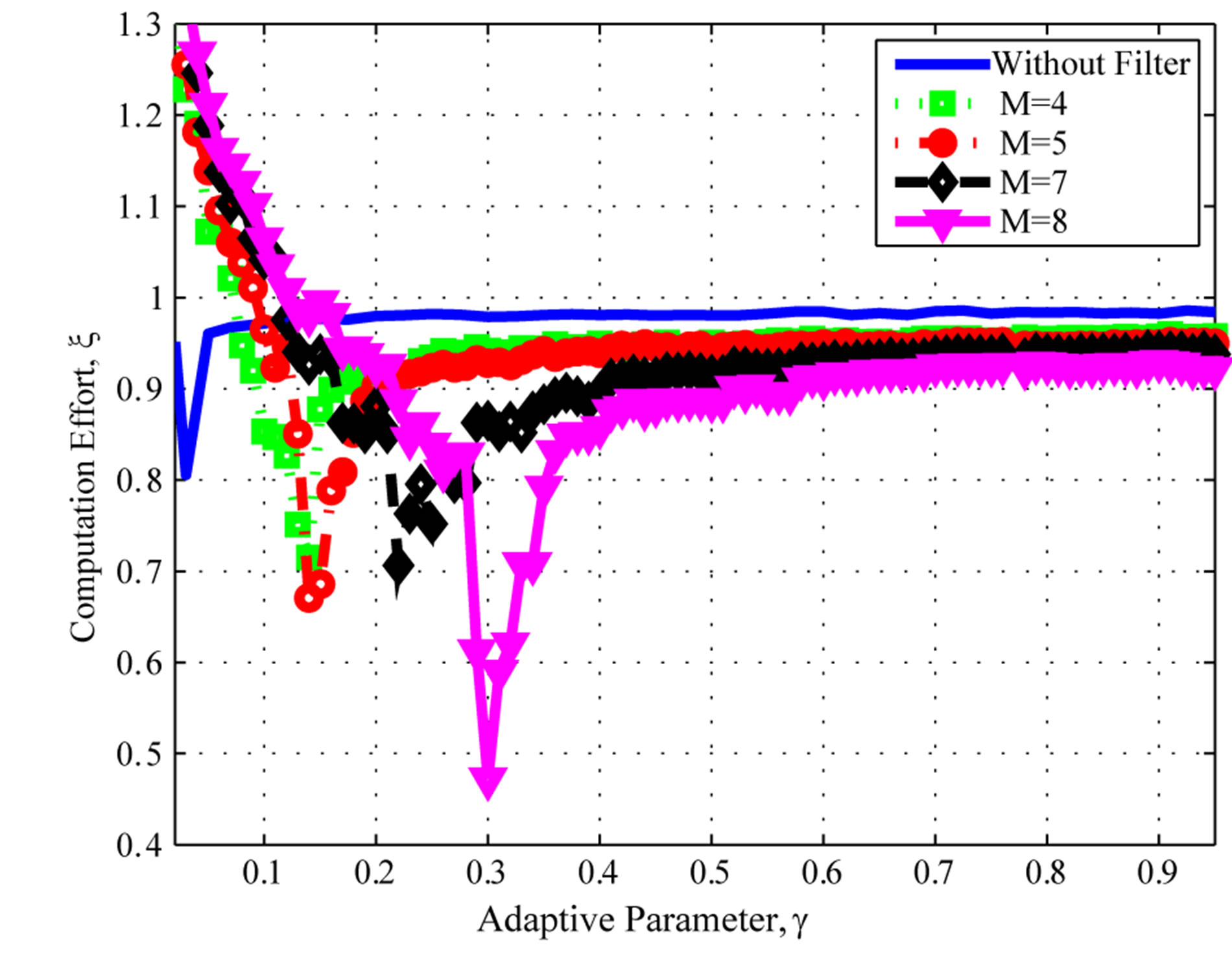
Figure 2 depicts the computational effort for higher filter orders, . One can see that no additional improvement is obtained for orders higher than 9. The main reason is that the underlying process that generates the error sequence
  has a given internal memory, or process memory. Whenever a estimator, i.e. moving average filter, exceeds the process memory, the estimator will decrease its performance [18].
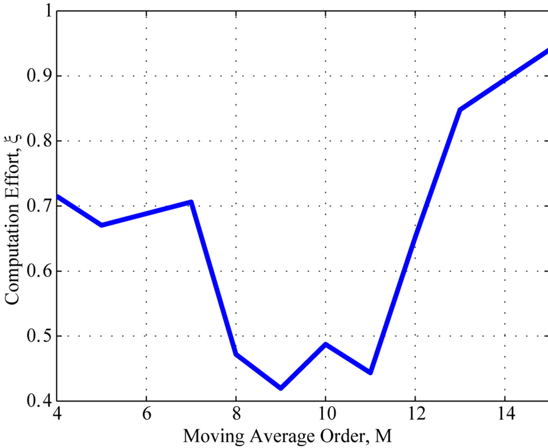
In order to illustrate the impact of the filter order on the computation effort, Figure 3(a) shows the computation effort for different filter order values. One can see the impact of the filter order in the performance, also noticing that is always improved with respect to unfiltered PIVI algorithm.
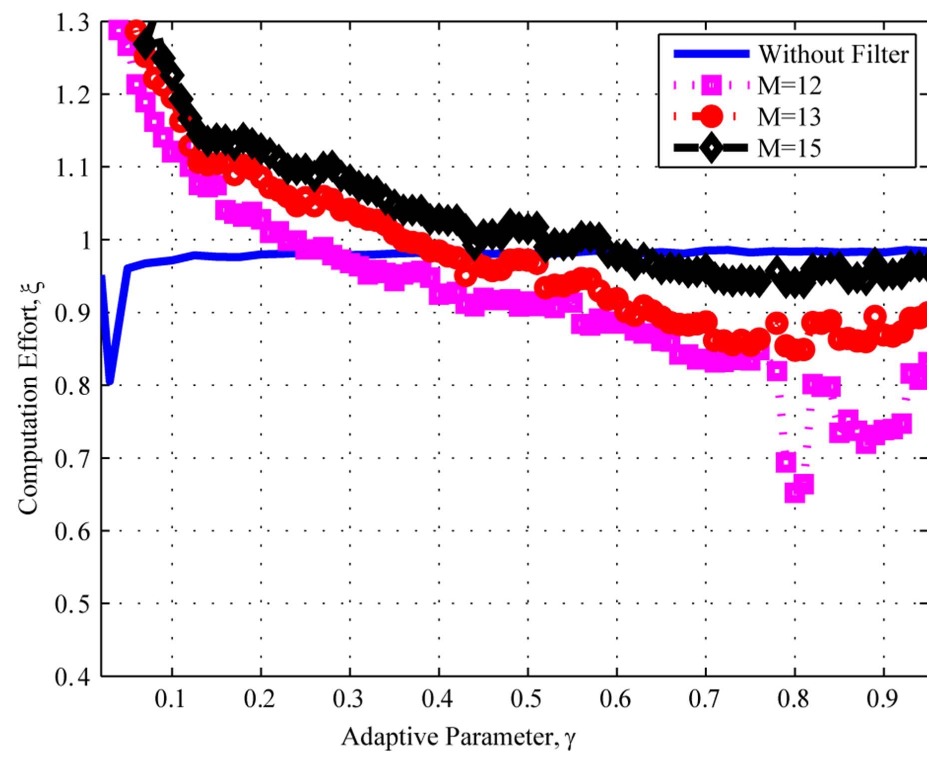
Figure 2. Computational effort: Poisson distribution, filter orders M = 12, 13, and 15.
 (a)
(a) (b)
(b)
Figure 3. The best adaptive parameter and computation effort as a function of the filter order M for Poisson distribution; (a) computation effort; (b) the best adaptive parameter γ.
Figure 3(b) presents the best adaptive parameter  for different values of filter order. One can notice on Figure 3(b) that the best value for the adaptive parameter
  spans over a wide range. Whenever the filter order is among
 ,
, 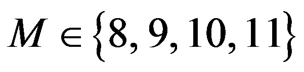 , the adaptive parameter
  has low sensibility, any value of
  in the range from 0.30 to 0.65, i.e.,
 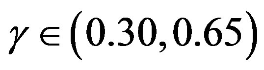 , would yield a significant improvement in the computational performance.
The first experiment suggests that the proposed method can provide significant savings in computational for problems with exogenous Poisson arrival processes. This is a very interesting results considering that such a class of problems tends to be very popular for queueing and manufacturing problems [16,19].
In the second experiment, the clients arrive in the first queue according to a geometric distribution with mean . Clients belonging to the second class arrive uniformly in the integer interval from 0 to 9. The geometric distribution is also truncated to retain a fraction of 0.9999 of the total transitions and then renormalized. Such a normalization is not needed for the uniform distribution. The joint arrival processes yields 660 possible transitions, hence
The classical VI algorithm converged in 104 iterations and applied an overall computational effort per state of .
.
Figure 4 depicts the overall computational effort  for parameter sequences of the type in (14), for different values of
 , normalized with respect to the overall VI effort
 . For this experiments, we make
 . The normalized computational effort for the proposed algorithm is plotted in Figure 4 as a function of the adaptive parameter,
 . One can see that, for a broad range of
 ,
,
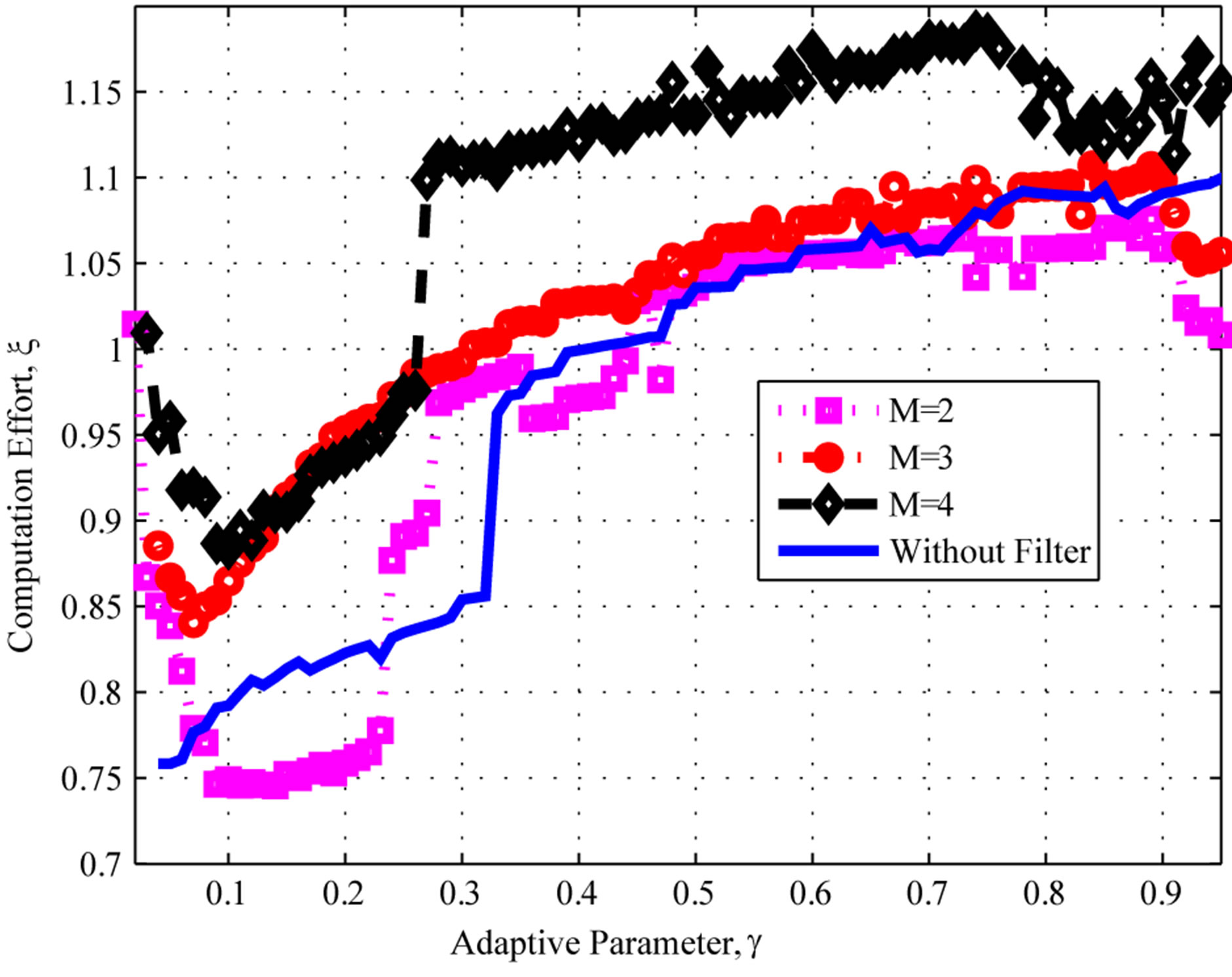
Figure 4. Computational effort: Geometric uniform distributions.
 , the computational effort is less than the classical VI algorithm. At the best point, the cost is about
  of the classical VI algorithm.
Note that the savings of the proposed algorithm for the second setting, though still appealing, are much less significant than those obtained for Poisson exogenous arrival processes. This suggests that more modest savings may be expected for uniform distribution settings. This is consistent with the results in [13], which suggest that PIVI algorithms tend to have a stronger performance for highly concentrated probability distributions, such as the Poisson distribution, while yielding less significant savings for distributions that are widely spread. Moreover, one can also notice that the moving average filter addition seems to have no significant effect on the results.
6. Concluding Remarks
This paper introduced a gradient adaptive version of the partial information value iteration (PIVI) algorithm introduced in [13] to the average cost MDP framework, with the addition of a moving average filter to smooth the empirical error sequence.
The proposed algorithm was validated by means of queueing examples, and presented consistent computational savings with respect to classical value iteration. Moreover, the proposed algorithm yielded consistent improvement over value iteration for a wide range of parameters, thus overcoming a shortcoming of a previous approach [14] that was overly sensitive to the parameter choice.
7. Acknowledgements
This work was partially supported by the Brazilian National Research Council-CNPq, under Grant No. 302716/ 2011-4.