1. Introduction
Vacation queues have been investigated for over two decades as a very useful tool for modeling and analyzing computer systems, communication networks, manufacturing and production systems and many others. The details can be seen in the monographs of Takagi [1] and Tian and Zhang [2], the survey of Doshi [3]. However, in these models, the server stops the original work in the vacation period and can not come back to the regular busy period until the vacation period ends.
Recently, Servi and Finn [4] introduced the working vacation policy, in which the server works at a different rate rather than completely stopping service during the vacation. They studied an M/M/1 queue with working vacations, and obtained the transform formulae for the distribution of the number of customers in the system and sojourn time in steady state, and applied these results to performance analysis of gateway router in fiber communication networks. During the working vacation models, the server can not come back to the regular busy period until the vacation period ends. Subsequently, Wu and Takagi [5] generalized the model in [4] to an M/G/1 queue with general working vacations. Baba [6] studied a GI/M/1 queue with working vacations by using the matrix analytic method. Banik et al. [7] analyzed the GI/ M/1/N queue with working vacations. Liu et al. [8] established a stochastic decomposition result in the M/M/1 queue with working vacations. Li et al. [9] established the conditional stochastic decomposition result in the M/G/1 queue with exponentially working vacations using matrix analytic approach.
For the batch arrival queues, Xu et al. [10] studied a batch arrival MX/M/1 queue with single working vacation. With the matrix analytic method, they derived the PGF of the stationary system length distribution, from which they got the stochastic decomposition result for the PGF of the stationary system length which indicates the evident relationship with that of the classical MX/M/1 queue without vacation. Furthermore, they found the upper bound and lower bound of the stationary waiting time in the Laplace transform order, from which they got the upper bound and lower bound of the waiting time.
In this paper, we study a batch arrival MX/M/1 queue with multiple working vacation. We obtain the PGF of the stationary system length distribution and the stochastic decomposition structure of system length which indicates the relationship with that of MX/M/1 queue without vacation. Although only the upper bound and lower bound of the stationary waiting time in the Laplace transform order are obtained in [10], we can obtain the exact LST of the stationary waiting time distribution.
The rest of this paper is organized as follows. In Section 2, the model of the MX/M/1 queue with multiple working vacation is described. In Section 3, we obtain the PGF of the stationary system length and its decomposition result which indicates the evident relationship with that of the classical MX/M/1 queue without vacation. Furthermore, we obtain the mean system length and several characteristic quantities. In Section 4, we obtain the LST of the stationary waiting time distribution. Numerical results for some special cases are presented in Section 5.
2. Model Description
Consider a batch arrival MX/M/1 queue with multiple working vacation. Customers arrive in batches according to a Poisson process with rate . The batch size
  is a random variable and

The PGF, the expectation and the second order moment of  are
are
 respectively.
Service times in the regular busy period follows an exponential distribution with parameter . Upon the completion of a service, if there is no customer in the system, the server begins a vacation and the vacation duration follows an exponential distribution with parameter
 . During a working vacation period, arriving customers are served at a rate of
 . When a vacation ends, if there are no customers in the queue, another vacation is taken. Otherwise, the server switches service rate from
  to
to , and a regular busy period starts. The LST’s of the service time distribution in a regular busy period and the service time in a working vacation time are
 respectively.
We assume that inter-arrival times, the service times and the working vacation times are mutually independent. Furthermore, the service discipline is first come first served (FCFS).
Let  be the number of customers in the system at time
  and
and

Then the process  is a two-dimensional Markov chain with the state space

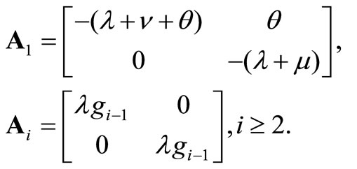
Using the lexicographical order for the states, the infinitesimal generator of the process  can be written as the Block-Jacobi matrix

where

Since  is reducible, it is found from Section 3.5 of Neuts [11] that the Markov chain is positive recurrent if and only if
 , that is,
 .
.
3. Stationary System Length Distribution
In this section, we derive the PGF of stationary distribution for . Let
. Let  be the stationary limit of the process
 . Assume that

Based on the stationary equations, we have
 (1)
(1)
 (2)
(2)
 (3)
(3)
 (4)
(4)
 (5)
(5)
Define the probability generating functions (PGF’s)

Then the PGF of stationary system length  can be written as

In order to prove Theorem 1 which states the stochastic decomposition structure of system length, the following lemma is necessary.
Lemma 1. The equation

has the unique root  in the interval
 .
.
Proof: We consider the function

For any , we have
 (6)
(6)
Therefore  is a concave function in the interval
 . Further,
 (7)
(7)
(6) and (7) indicate that the equation  has the unique root
  in the interval
 .
.
Remark 1. Lemma 1 in this paper is the same as Lemma 1 in Xu et al. [10]. But the proof in this paper is simpler than the proof in [10].
We have the following Theorem which proves the stochastic decomposition structure of system length.
Theorem 1. If  and
and , the stationary system length
  can be decomposed into the sum of two independent random variables,

where  is the stationary system length in corresponding classical MX/M/1 queue without vacation and has the PGF
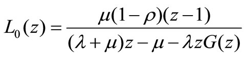 (8)
(8)
 is the additional system length and has the PGF
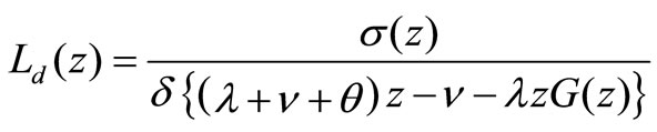 (9)
(9)
where

and

Proof: Multiplying the Equation (2) by  and each equation of (3) by
  and summing up these equations, we have

After calculations, we have

Therefore, we obtain
 (10)
(10)
Since  is an analytic function in
 , wherever the right-side of (10) has zeros in
 , so must the numerator. From Lemma 1, the denominator of
  is equal to 0 if
 , so does the numerator. Substituting
  into the numerator of the right-hand side of (10), we have
 (11)
(11)
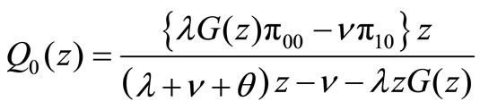
Substituting (11) into (10), we have
 (12)
(12)
Similarly, multiplying the Equation (4) by  and each equation of (5) by
  and summing up these equations, we have

After calculations, we have

Therefore, we obtain
 (13)
(13)
Since  is finite and
  , we have
 (14)
(14)
Substituting  into (12), we have
 (15)
(15)
Using (14) and (15), we have
 (16)
(16)
Using (10) and (16), we finally obtain
 (17)
(17)
where

Using the condition that  and L’Hospital’s rule, we have

Obviously, the numerator and the denominator of the above expression are both positive since  and
and . Furthermore, we have
 (18)
(18)
where

Substituting the expressions of  into (17), we finally obtain
 (19)
(19)
Since ,
,  is a PGF. Therefore, we completes the proof of Theorem 1.
From Theorem 1, we can obtain two important characteristic quantities in the following two Corollaries.
Corollary 1. The mean of stationary system length  is given by

Proof: From (8), we have

From (9), we have

Therefore, we obtain

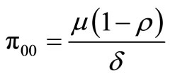
Corollary 2. The probability  that the system is in a working vacation period and the probability
  that the system is in a regular busy period are given by

respectively.
Proof: Using (12) and (18), we have

then we have

4. Stationary Waiting Time
In this Section, we can obtain the LST of the stationary waiting time of an arbitrary customer. Let  and
and  denote the stationary waiting time of an arbitrary customer and its LST, respectively.
Theorem 2. If  and
and ,
,  is given by
 (20)
(20)
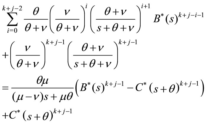
Proof: To compute , we consider three possible cases as follows.
Case 1: A batch of customers including the tagged customer arrive in the state . There are
  customers in front of this batch of customers in the system. In this case, a tagged customer’s waiting time in this batch is the sum of the service times of
  customers outside of his batch and a period of waiting time inside of his batch. Let
  be the probability of the tagged customer being in the jth position of arriving batch. Using the result in renewal theory (Burke [12]), we have

Since all the customers are served at the normal service level, the tagged customer’s waiting time conditioned that a batch of customers arrive in the state , denoted by
 , has the LST

Therefore, we have
 (21)
(21)
Case 2: A batch of customers including the tagged customer arrive in the state . There are
  customers in front of this batch of customers in the system. If the tagged customer is the jth position in his batch, the LST of waiting time of the tagged customer is given by
Let  and
and  denote the tagged customer’s waiting time conditioned that a batch of customers arrive in the state
  and its LST, respectively. Then we have
 (22)
(22)
Case 3: A batch of customers including the tagged customer arrive in the state . The tagged customer’s waiting time is equal to the waiting time inside of his batch. Therefore, the tagged customer’s waiting time conditioned that a batch of customers arrive in the state
 , denoted by
 , has the LST

From (21), (22) and (23), we finally obtain

Remark 2. We can obtain the mean waiting time of an arbitrary customer,  by differentiating (20) and substituting
 . On the other hand, the mean waiting time of an arbitrary customer,
  , can also be obtained by Little’s formula, that is,

However, in order to obtain the higher moments of the waiting time of an arbitrary customer, 
 , we must differentiate (20)
  times and substitute
  .
.
Remark 3. If , our model reduces to a batch arrival MX/M/1 queue with multiple vacation. If the batch size of arrivals is always equal to 1, that is,
  , our model reduces to an M/M/1 queue with multiple working vacation studied in Servi and Finn [4] and Liu et al. [8]. These results correspond to the known results in existing literature.
5. Numerical Results
In Section 3 and Section 4, we obtain the mean system length and the mean waiting time of an arbitrary customer. In this section, we assume that the arrival batch size  follows a geometric distribution with parameter
 , that is,
 . Then it is easy to verify that

First, we consider an MX/M/1 queue with multiple working vacation where the system parameters are . In Figure 1, we demonstrate the effect of the service rate in the working vacation period
  on the mean system length
  for different
 . Figure 1 indicates that
  decreases as
  increases when
  is equal to 2, 3 and 4, respectively. On the other hand, if
  is fixed,
  increases as
  increases, that is,
  increases.
Secondly, we assume that . In Figure 2, we demonstrate the effect of
  on
on  for different vacation rate
 . Figure 2 indicates that
  decreases as
  increases when
  is equal to 0.5, 1.0 and 1.5, respectively. On the other hand, if
  is fixed,
  decreases as
  increases.
Thirdly, in Figure 3, we present the comparison of three queueing model, that is, the MX/M/1 queue without vacation, the MX/M/1 queue with multiple vacation and the MX/M/1 queue with multiple working vacation. Assume that  for the MX/M/1 queue with multiple working vacation. Figure 3 indicates that
  and
and  increase as
  increases. On the other hand,
  and
and  of MX/M/1 queue

Figure 1. E(L) versus v for different g.

Figure 2. E(L) versus v for different θ.
without vacation are shortest and those of the MX/M/1 queue with multiple vacation are longest, which is identical with the intuition. Furthermore, Figure 3 indicates that  and
and , which is a well known result for batch arrival queues.
6. Conclusion
This paper studied the MX/M/1queue with multiple working vacation. We obtained the PGF of the stationary system length distribution and the stochastic decomposition structure of system length which indicates the relationship with that of the MX/M/1 queue without vacation. Performance indices such as the mean of stationary system length, the probability that the system is


Figure 3. E(L) and E(W) versus ρ for different queueing model.
in a working vacation period and the probability that the system is in a regular busy period were also presented. Further, we obtained the LST of the stationary waiting time distribution of anarbitrary customer.We obtained the mean system length and the mean waiting time. Some numerical results for special cases showed efficiency of service in this multi-purpose batch arrival model.
7. Acknowledgements
We would like to thank the referees for valuable comments.