1. Introduction
Consider the following initial-boundary value problem of pseudo-hyperbolic equation
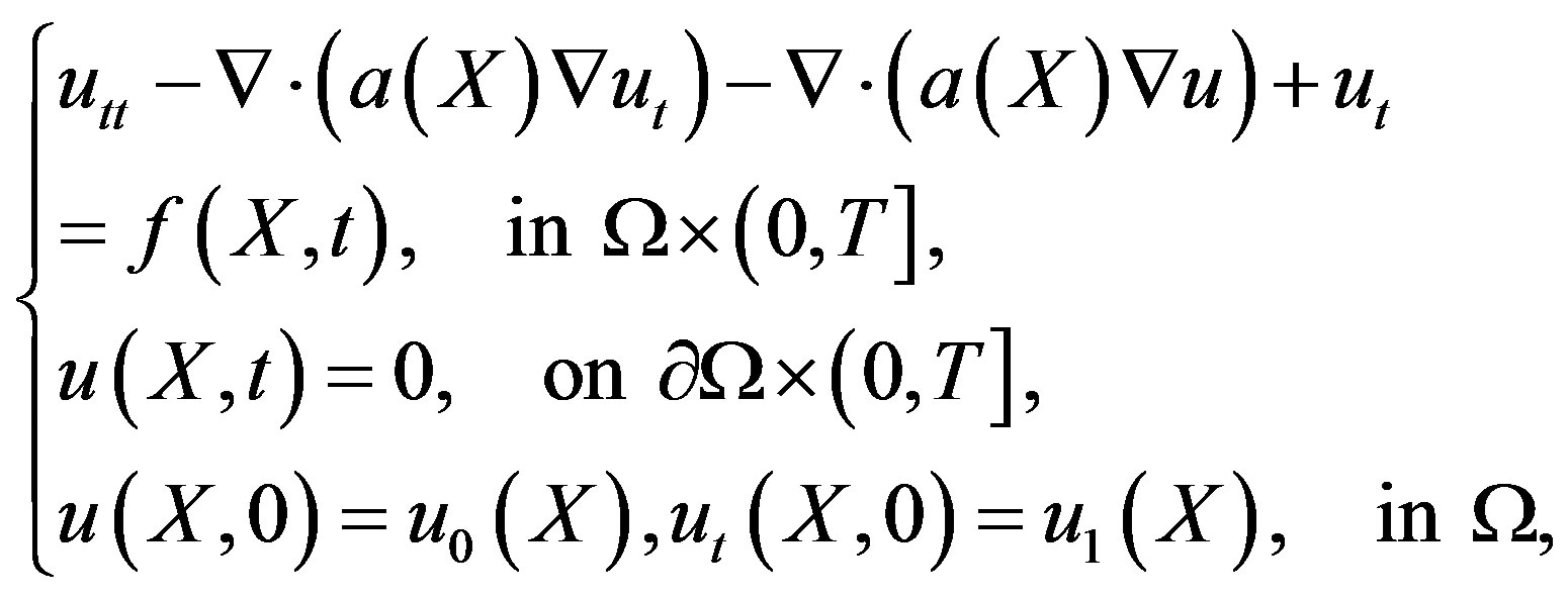 (1)
(1)
where 
 is bounded convex polygonal domain in
  with Lipschitz continuous boundary
 .
.
 is smooth function with bounded derivatives,
 ,
,  and f are given functions, and
 for positive constants
  and
and .
.
The pseudo-hyperbolic equation is a high-order partial differential system with mixed partial derivative with respect to time and space, which describe heat and mass transfer, reaction-diffusion and nerve conduction, and other physical phenomena. This model was proposed by Nagumo et al. [1]. Wan and Liu [2] have given some results about the asymptotic behavior of solutions for this problem. Guo and Rui [3] used two least-squares Galerkin finite element schemes to solve pseudo-hyperbolic equations.
On the other hand, H1-Galerkin mixed finite element method (see [4]) has been under rapid progress recently since this method has the following advantages over classical mixed finite element method. The method allows the approximation spaces to be polynomial spaces with different orders without LBB consistency condition and there is no requirement of the quasi-uniform assumption on the meshes. For example, Pani [4,5] proposed an H1-Galerkin mixed finite element procedure to deal with parabolic partial differential equations and parabolic partial integro-differential equations, respectively. Liu and Li [6,7] applied this method to deal with pseudohyperbolic equations and fourth-order heavy damping wave equation. Further, Shi and Wang [8] investigated this method for integro-differential equation of parabolic type with nonconforming finite elements including the ones studied in [9,10].
It is well-known that the convergence behavior of the well-known nonconforming Wilson element is much better than that of conforming bilinear element. So it is widely used in engineering computations. However, it is only convergent for rectangular and parallelogram meshes. The convergence for arbitrary quadrilateral meshes can not be ensured since it passes neither Irons Patch Test [11] nor General Patch Test [12]. In order to extend this element to arbitrary quadrilateral meshes, various improved methods have been developed in [13-24]. In particular, [19-24] generalized the results mentioned above and constructed a class of Quasi-Wilson elements which are convergent to the second order elliptic problem for narrow quadrilateral meshes [23].
In the present work, we will focus on H1-Galerkin nonconforming mixed finite element approximation to problem (1) under arbitrary quadrilateral meshes. We firstly prove the existence and uniqueness of the solution for semi-discrete scheme. Then, based on a very special property of the quasi-Wilson element i.e. the consistency error is one order higher than interpolation error, we deduce the optimal order error estimates for semidiscrete scheme directly without using the generalized elliptic projection which is a indispensable tool in the tradition finite element methods.
This paper is arranged as follows. In Section 2, we briefly introduce the construction of nonconforming mixed finite element. In section III, we will discuss the H1-Galerkin mixed finite element scheme for pseudohyperbolic equations. At last, the corresponding optimal order error estimates are obtained for semi-discrete scheme.
2. Construction of Nonconforming Mixed Finite Element
Assume  to be the reference element in the
  plane with vertices
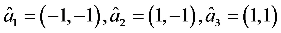 and
and .
.
Let  and
and  be the four edges of
 .
.
We define the finite elements  by
by


where ,
,  ,
,  ,
,


and
When , it is the so-called Wilson element.
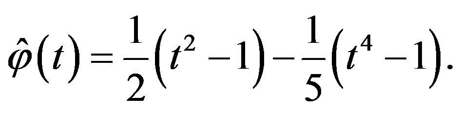
The interpolations defined above are properly posed and the interpolation functions can be expressed as

and

Given a convex polygonal domain , Let
, Let
 be a decomposition of
  such that
satisfies the regularity assumption [11], where K denotes a convex quadrilateral with vertices
 ,
, 
 is the diameter of the finite element K.
Then there exists a invertible mapping 

The associated finite element space  and
and  are defined as

and

Then for all we define the interpolation operators
  and
and  by
by
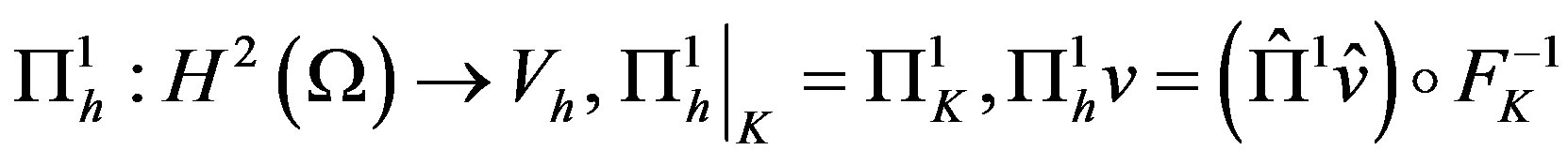
and

Let  be the set of square integrable functions on
  and
and  the space of two dimensional vectors which have all components in
  with its norm
 . Let
. Let  be the space of vectors in
 which has divergence in
  with norm
 denotes the
  inner product. For our subsequent use, we also use the standard sobolve space
  with a norm
  Especially for
 , we denote
  and
and
Throughout this paper, C denotes a general positive constant which is independent of h.
3. Nonconforming H1-Galerkin Mixed Finite Element Method for the Semi-Discrete Scheme
Let  and
and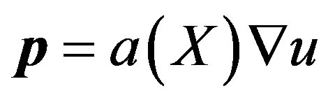 , then the corresponding weak formulation is: Find
  , such that
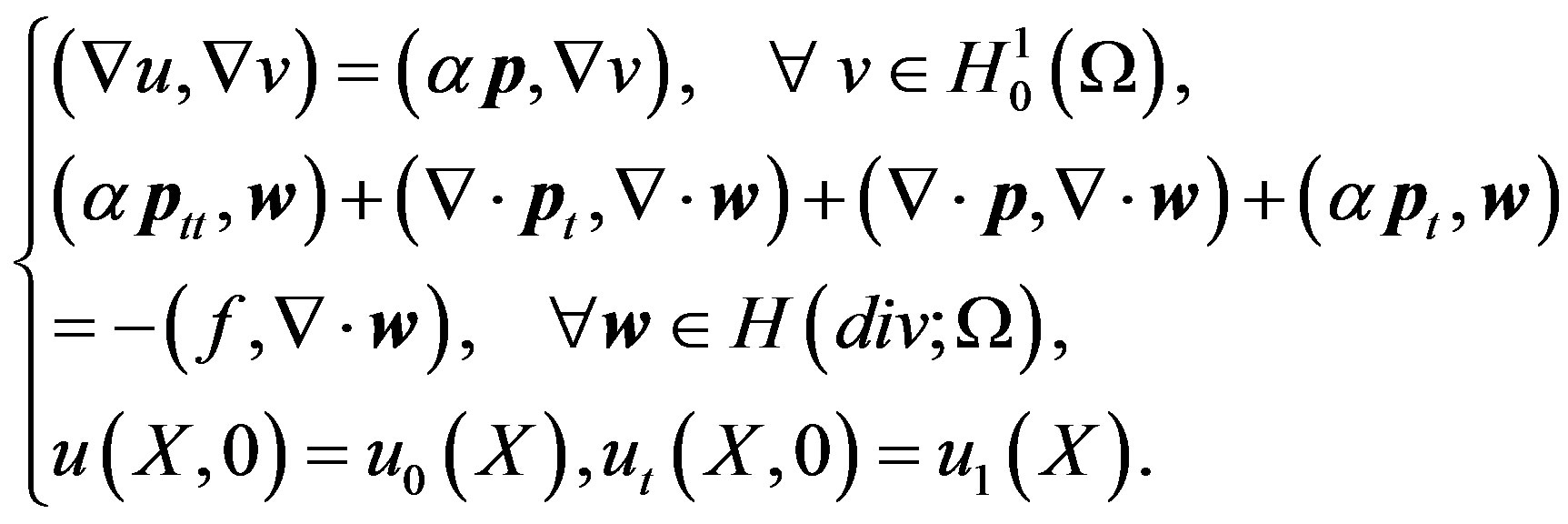 (2)
(2)
The corresponding semi-discrete finite element procedure is: Find , such that
 (3)
(3)
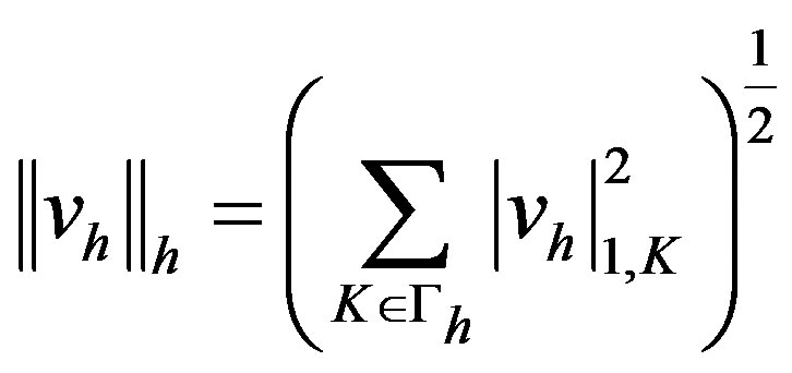
For all , we define
and
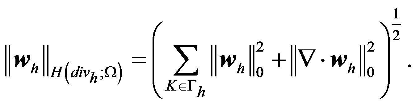
It is easy to see that  and
and  are norms of
 and
and , respectively.
Theorem 1. Problem (3) has a unique solution.
Proof. Let  and
and  the basis of
  and
and
 . Suppose that

then (3) can be written as
 (4)
(4)
where


Sine (4) gives a system of nonlinear ordinary differential equations (ODEs) for the vector function  and
and , by the assumptions on
  and the theory of ODEs, it follows that
  and
and  has the unique solution for
  (see [25]). Therefore the proof is complete.
4. Error Estimates
In order to get the error estimates the following lemma which will play an important role in our analysis and can be found in [24].
Lemma 1. For all , then there holds

where  denotes the outward unit normal vector to
 .
.
Now, we will state the following main result of this paper.
Theorem 2. Suppose that  and
and  be the solutions of the (2) and (3), respectively,
 ,
,  and
and
 , then we have
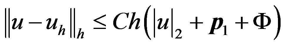 (5)
(5)
and
 (6)
(6)
where
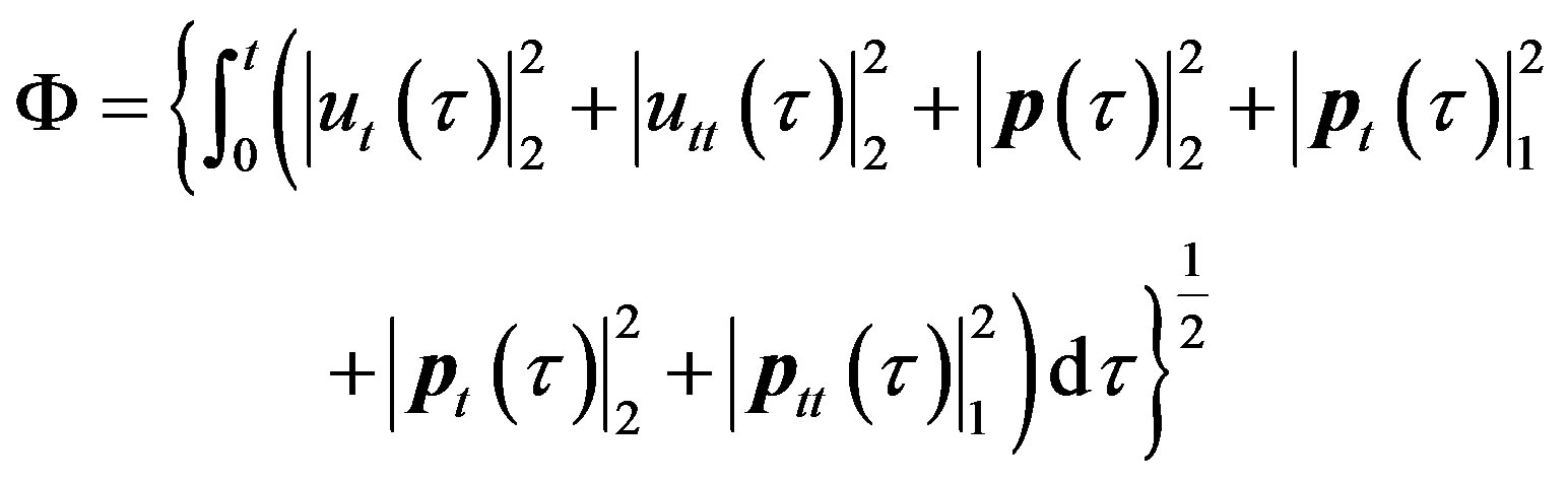 .
.
Proof. Let 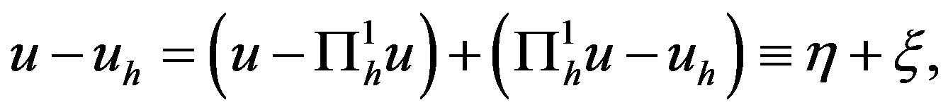

It is easy to see that for all , there hold the following error equations
 (7)
(7)
Choosing  in (7(a)) and using the CauchySchwartz’s inequality yields
 (8)
(8)
Further, choosing  in (7(b)) leads to
 (9)
(9)
For the right side of (9), applying  -Young’s inequality and noting that
  is a smooth function with bounded derivatives, we get
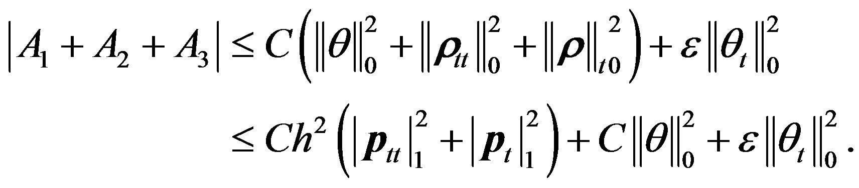 (10)
(10)
 (11)
(11)
By Lemma 1 and  -Young’s inequality, we have
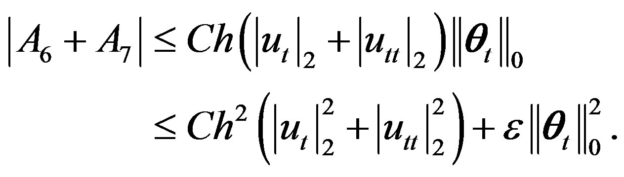 (12)
(12)
Choosing small  and combining (9)-(12), we can derive
 (13)
(13)
Integrating the both sides of (13) with respect to time from 0 to t, by Gronwall’s lemma and noting  , we obtain
 (14)
(14)
together with (8), there yields
 (15)
(15)
Finally, by use of the triangle inequality, (14) and (15), we get (5) and (6). The proof is completed.
5. Acknowledgements
This research is supported by National Natural Science Foundation of China (Grant No.10971203); Tianyuan Mathematics Foundation of the National Natural Science Foundation of China (Grant No.11026154) and the Natural Science Foundation of the Education Department of Henan Province (Grant Nos.2010A110018; 2011A110020).
NOTES