Numerical Solution of Advection Diffusion Equation Using Semi-Discretization Scheme ()
1. Introduction
The advection diffusion equation (ADE) is the model that can be used for simulation natural processes. Two categories of the advection-diffusion equation: advection is first due to the movement of materials from one region to another; the second category is called diffusion which is due to the movement of materials from higher concentration to low concentration. This mathematical model has a wide range of applications in natural science and engineering. These applications include where simulation techniques are useful for transport of air, river water, adsorption of pollutants in soil, food processing, modeling of the biological system, finance, electromagnetism, fluid mechanics structural dynamics, quantum physical process, etc. The analytical and numerical solutions along with an initial and two boundary conditions help to comprehend pollutant concentration distribution behavior through an open medium like rivers, air, lakes, and porous medium. Various works have been appeared to solve and use this equation in their simulation using finite difference methods [1] [2] [3]. Numerical Solution of the 1D advection-diffusion Equation solved using standard and nonstandard Finite Difference Schemes [4]. The significant application of the linear advection diffusion equation lies in fluid dynamics, heat transfer, and mass transfer [5]. Researchers examine numerical solution of Advection Diffusion Equation using operator splitting method [6]. These methods have been implemented by a characteristic method with cubic spline interpolation (MOC-CS) and Crank-Nicolson (CN) finite difference scheme. Obtained results were compared with analytical solutions. It is seen that the implemented method has lower error than other methods also produces accurate results even when the time steps are great. The linear advection diffusion equation (ADE) is a model which describes the contaminant transport due to the combined effect of advection and diffusion in a porous media [7]. In this study, the advection diffusion equation is solved by explicit finite difference schemes and investigates a different approach, the semi-discretization method: a spatial variable which yields a system of ODE with the temporal independent variable. We solve this system of ODE’s by Euler’s method and develop an algorithm of the Euler method for the system of ODE’s and implement it for the computation of the concentration
.
2. Advection Diffusion Equation
We consider the following partial differential equation, which has both an adventive and diffusive terms together.
(1)
with initial condition:
.
And boundary conditions:
where
are concentration values and
is the unknown solution being investigated which indicates concentration,
is the velocity of the medium in the x direction,
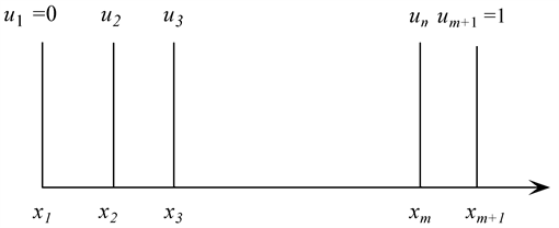
is the diffusion coefficient. To introduce numerical scheme for Equation (1), an advection diffusion problem whose general solution [8] [9] [10] is (Figure 1)
(2)
3. Numerical Methodology
In mathematics, our goal is to approximate the solution of the differential equations.
![]()
Figure 1. The general solution of the advection diffusion equation.
This gives a large algebraic system of equations to be solved in replace of the differential equation, which can be easily solved [11] [12] on a computer by Matlab code.
3.1. Computational Grid
We consider some simple space discretization on a uniform grid. We divide the spatial interval
into
equal sub-interval such that
with
and
.
Approximations
are found by replacing the spatial derivatives by difference quotients. we also divide the time interval
into
equal subinterval such that
with
,
and
. For purpose of the notation
and
.
This gives a finite difference discretization in space. Setting
.
Therefore, we get a system of ordinary difference equations (ODEs) of (1.1)
(3)
with a given initial value
.
3.2. Discretization of Explicit Finite Difference Scheme (ECDS)
To approximate the solution to Equation (1) using the Explicit Centered Difference Scheme, we use the following approximations
(a)
(b)
(c)
where
is the spatial step,
is the time step, m and n is spatial and temporal node respectively. Substituting Equation (a), (b), (c) in Equation (1) and solving
for unknown
. We obtain
where
and
. Stability condition
&
.
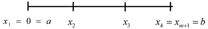
3.3. Spatial Discretization Technique for ADE and Solved by Euler Method
We consider the following figure for ADE (Advection Diffusion Equation).
We draw vertical grid line as shown in the picture. These lines are parallel to the t-axis and cross the x-axis in
,
.
,
.
In semi-discretization method (SDM), we assume that the PDE system with its boundary conditions has spatially discretized, and thus we focus on ODE system
, representing semi-discrete advection-diffusion problems.
This equation is same as Equation (2). Now Consider ADE (1) with
and
.
We introduce the function of one variable:
,
.
Now approximate the first derivative and second derivative
and
respectively as:
(d)
(e)
This gives the semi-discrete form of (1)
(4)
Setting
We get,
So, we obtain a linear system of ordinary differential equations (ODE’s) of the type.
Now, we get with time step
for the numerical solution
which is the semi discretization using Euler method of
.
4. Numerical Result’s and Discussion
4.1. Algorithm for the Semi Discretization of ADE Solved by Euler Method
To approximate the solution to the partial differential equation
Input: dt, dx, constant co-efficient
,
, the left and right end point
of
;
, the right end point of
.
Output: approximation
to
for each
,
.
Step 1: set
Step 2: for
Step 3:
Step 4-Step 6: (solve a tri-diagonal linear system)
Step 4: Construct matrix A and B
Set,
Boundary
(Unknown solution for first time step)
Step 5: For
Set
;
Output
,
Step 6: Stop (the procedure complete)
4.2. Case Study
Numerical implementation of Euler method [10] [11]: our solving equation (1):
initial condition:
Boundary condition:
We will solve numerically for the concentration u using matrix system of equation.
Suppose we use 4 grid points
i.e.
in this example.
We let,
, Solution for concentration vector
at time
.
The boundary condition gives
and
.
We can rewrite general nth term in Equation (4) to required Euler method of advection diffusion equation.
4.3. Semi Discretization Scheme for ADE Solved Using Euler Method
For this case the time step is increased to
,
, and the parameter
and
,
known as advection equation number and
known as diffusion term. Regarding this application, (Figure 2)
Summary of elapsed time for different temporal grid point present below:
![]()
Figure 2. The concentration distribution for
at different time of Euler and ECDS.
5. Error Analysis and Convergence
5.1. Error Analysis
The comparison of relative error for two finite difference schemes as a function of time is shown in Figure 3. Two different curves show relative error for Explicit (red) and Euler (blue). We found the relative error for ECDS remains below 0.0009 and the relative error for Euler remains below 0.0011.
5.2. Convergence
Figure 4 illustrates the convergence of relative error by the scheme FTCS techniques. In this figure, numerical computation of ADE is presented by using explicit finite difference methods by FTCS and compared with an exact solution of
![]()
Figure 3. Plot shows Relative error of ADE for both schemes.
![]()
Figure 4. Plot shows Convergence of relative error for ECDS.
the ADE. A good agreement between the numerical solutions and the analytical solutions is obtained and the error becomes clear when using large size step for the time.
Figure 5 presents the convergence of semi discretization by Euler for ADE with respect to time. It can be seen that, the relative error rate of the convergence curves for the Euler scheme with respect to time. This figure shows a very good rate of convergence.
5.3. Problem Discussion
Figure 6 describes the concentration distribution profile as a function of distance. Different curves represent concentration distribution profiles at different times starting from
to
. The plot marked by “red curved”
![]()
Figure 5. Plot shows error rate of convergence for Euler scheme.
![]()
Figure 6. Plot shows concentration distribution at different time.
represents the concentration is high for 10 seconds and the green curve shows that concentration is decreased for 20 seconds. The curve marked by “blue” represents concentration is high for 30 seconds and. The plot marked by “yellow” represents concentration is high for 50 seconds we can see that when time is increased concentration profile is decreasing. As can be seen in Figure 6, five curves show concentration distribution profiles for different times, advection, and diffusion parameter as a function of distance.
Similarly, we observe the above figure with the concentration distribution profile for different distances is decreased in a position with respect to time in Figure 7.
Figure 8 represents the concentration profile for different velocities and different diffusion coefficients regarding distances. Different curves show concentration profiles for different applied velocities and diffusion rates. If we vary
![]()
Figure 7. Plot shows concentration distribution at different position.
![]()
Figure 8. Plot demonstrated varying advection & diffusion rate a time
.
![]()
Figure 9. The plot demonstrated varying diffusion rate a time
.
both velocity and diffusion coefficient at t = 20 secs, the solutions appeared which can be seen in Figure 8.
Similarly, concentration profile by solving numerically at a different diffusion rate can be seen in Figure 9 where the maximum concentration profile is shown at time
.
6. Conclusion
We present numerical solutions with exact solutions for the advection-diffusion equation with an initial condition and two boundary conditions by using ECDS and semi discretize method. A numerical study of the ADE has been presented graphically for two different schemes. The numerical solution of ADE by semi-discretization scheme shows a good agreement with the exact solution as well as for ECDS. Though, ECDS seems a more efficient scheme in terms of elapse timing; we compute the relative errors for two different schemes, both schemes show a very good rate of convergence. In comparison to Euler’s method, ECDS shows less error, which is obvious. Semi discretize methods have to deal with a large number of systems of ordinary differential equations in comparison with ECDS. In our next work, we would like to upgrade this work with higher-order accuracy.