Evaluation and Comparison of Different Machine Learning Methods to Predict Outcome of Tuberculosis Treatment Course ()
1. Introduction
Over recent years, Tuberculosis has been considered, particularly in low and middle-income countries as a global public health concern with the estimated two million deaths annually [1,2]. Up to 50% of all patients with TB do not complete treatment and fail to adhere to their therapy [3]. It has been estimated that in industrialized countries non-completion of treatment is around 20% [4] and according to the Centre of Disease Control and Prevention in the United States, 25% of patients fail to complete their chemotherapy [5]; in other words, the proportion of patients with active disease who completes therapy under standard conditions ranges from as little as 20% - 40% in developing countries to 70% - 75% in the USA [6]. Noncompliance is a significant factor leading to the persistence of tuberculosis in many countries and the consequences of this well recognized fact are prolonged infectiousness, relapse, prolonged and more expensive therapy due to multidrug resistance TB and death [7]. It has been revealed that noncompliance is associated with a 10-fold increase in the incidents of poor results from treatment and accounted for most treatment failures [8]. It is the most serious problem hampering tuberculosis treatment and control as patients with active disease who are non-compliant, sputum conversion to smearnegative will be delayed and relapse rates will be 5 - 6 times higher and drug resistance may develop [6]. That is, TB patients remained in the pool of active cases will increase the development of TB among latent cases who are prone to be infected or affected. This threats public health and makes huge costs that can be spent to improve public health improvement and promotion instead.
DOTS (directly observed treatment, short course) which is current international control strategy for TB control involves the case detection and completes the entire course of treatment successfully. In 2006, in order to improve DOTS quality, World Health Organization (WHO) has designed “Stop TB” Plan [2]. In this plan, it has been highlighted that health care services should identify and concentrate on interruption factors that halt TB treatment. Supervision which plays important role in patient treatment adherence and drug resistance prevention must be carried out in a context-specific and patient-sensitive manner.
Although WHO has highlighted the necessity of improving the quality of DOTS in terms of supervision and patient support in the “Stop TB” plan, there is no specific way to measure how intensive health providers’ support and supervision should be and to whom of TB cases it should be provided. To make this clear, we may require a tool to predict the patient destination regarding TB treatment course completion. The tool may identify high risk TB patients for treatment course non-compliance as it is impossible to serve all TB patients with active supervision and support due to the cost consideration and limited resources. This may be used to define the level of supervision and support each patient needs based on the predicted outcome by an accurate predictive model. Currently, no system is available to estimate TB treatment course through using features of TB patients and designing a systematic method to predict the given outcome.
For the prediction of tuberculosis treatment course completion, the defined outcome related to each record of TB patient contains five potential classes: cure and completed treatment (desirable outcomes), failure, quit, and death (undesirable outcomes) [9]. Patients who are classified with undesired outcomes need more supervision and support. Public health interventions for TB control need to be set according to how many of TB patients would shift to unwelcome outcomes.
Making sure that TB patients finish the treatment course entirely is a main step to TB control and public health promotion. Actually, here the main question of concern is “can new TB cases at risk of failing in treatment course completion identified from their early registration”? For this purpose, machine learning methods have been already applied and they worked properly according to previous studies [10,11]. They infer a model through being trained by a set of historical examples in frame of data categories; thus, new examples with unknown classes could be assigned to one or more classes by pattern matching within the developed valid model [12].
This work used machine learning algorithms to achieve six predictive models of a crucial real-world problem which offer the medical research community a valid alternative to manual estimation of risky TB patients to quit or fail treatment course completion. This recognizes TB patients whom supervision in frame of DOTS therapy needs to be more active as they are risky for treatment course interruption.
2. Methods and Algorithms
2.1. Correlation Analysis
In the case of a large dataset, learning the dataset is not useful unless the unwanted features are removed since an irrelevant and redundant feature does not add anything positive and new to the target concept [13]. To identifying influential predictors, a bivariate correlation is used which is a correlation between two variables including independent and dependent parameters by calculating the correlation coefficient “r” [14]. As there is no specific prediction and hypothesis two-tailed test is carried out.
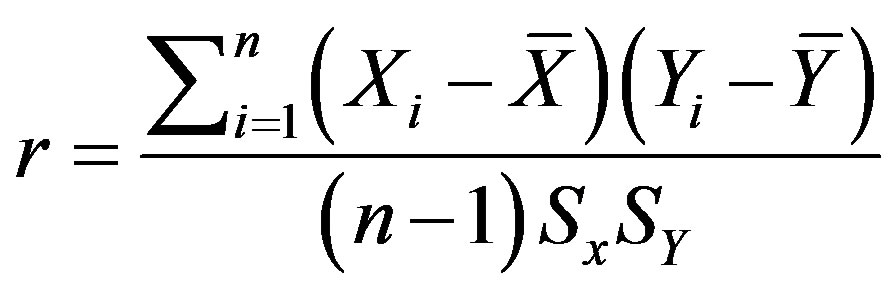
Suppose we have got two variables X (list of features) and Y (class), an optimal subset is always relative to a certain evaluation function. To discover the degree to which the variables are related, correlation criteria are applied [15]. It reflects the degree of linear relationship between two variables ranging from +1 to −1. A perfect positive linear relationship between variables is shown by +1; however, −1 implies an entire negative linear association. The following formula (1) is used to calculate the value of r:
 (1)
(1)
where there are two variables X and Y and their means X, Y and standard deviations including SX and SY respectively; n is the number of TB instances. The correlation coefficient can be tested for statistical significance using special t-test through following formula.
 (2)
(2)
Degree of freedom for correlation coefficient calculation is equal to n − 2. From a t-table, we would find significant relationship between each of variables X and Y (P < 0.05).
2.2. Problem Modeling
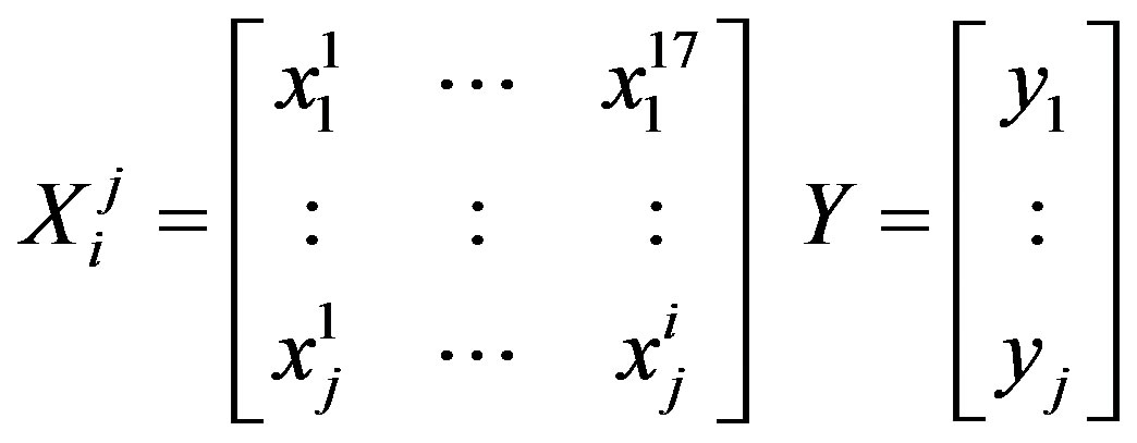
To achieve the aim of this work, we evaluate a number of well-known classification algorithms on TB treatment course completion. In fact, prediction can be viewed as the construction and use of a model to assess the class of an unlabeled sample, or to evaluate the value or value ranges of an attribute that a given sample is likely to have [16]. To train every of applied algorithms, we set a big matrices as follows:
 (3)
(3)
where X is a big matrice which is used to train the given algorithm by using train set in which i would be the ith number of samples and j is the jth number of predictor.  in our training set would be
  and in applied testing set has been
 . Y which is the dependent variable of TB treatment course in both training and testing sets addresses five classes where a label of “1” implies that TB case got cured and “2” means that s/he has completed the treatment course entirely; whilst a label of “3”, “4”, and “5” means that the patient belongs to the undesirable class such as quitting, failing the treatment course, or dead respectively.
Having compared the pros and cons of machine learning methods, to carry out the considered prediction task in this study six classifiers including decision tree (DT), Bayesian network (BN), logistic regression (LR), multilayer perceptron (MLP), radial basis function (RBF) and support vector machine (SVM) were selected. Next section is brief explanation about each of these selected classifiers. As shown in Figure 1, the dataset was split

Figure 1. Schematic presentation of applied methodology of model development and validation process. In order to develop accurate predictive or classification models, firstly data of TB patients (in a huge matice with 6450 rows and 18 vectors) are divided as training and testing sets. Training set is used to learn data and build models through applying 6 algorithms including decision tree (DT), support vector machine (SVM), logistic regression (LR), Bayesian network (BN), radial basis function (RBF), and artificial neural network (ANN). To check the validity and accuracy of developed models, testing set is applied.
into training (two-third) and testing (the other one-third) datasets each containing seventeen significantly correlated attributes and the outcome variables for every record without any missing data. The six above named classifiers were applied to the training dataset to estimate the relationship among the attributes and to build predictive models. Afterwards, the testing dataset which was not used to model inference was utilized to calculate the predicted classes and compare the predicted values with the realones available in the testing dataset. The model which is the most fitted and accurate one will be selected to predict the outcome of Tb treatment course for new TB cases.
2.3. Modeling Algorithms
2.3.1. Decision Tree
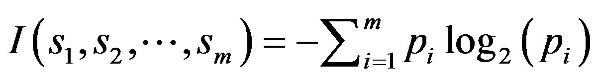
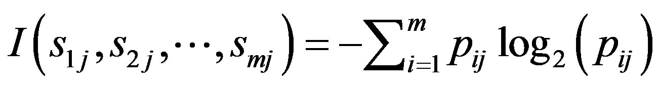
The decision tree is a nonparametric estimation algorithm that input space is divided into local regions defined by a distance measure like the Euclidean norm; it is a flowchart-like tree structure where the internal node, branches, and leaf node means concepts associated with our training tuples. In this hierarchical data structure, the local region is identified in a sequence of recursive splits that in a smaller number of steps by implementing divideand-conquer strategy. This powerful classifier is famous for its intuitive explainability [17]. In this research, C4.5 classification task-oriented algorithm has been applied through calculating:
 (4)
(4)
 (5)
(5)
where  is the probability that an instance belongs to class
 . Having calculated the entropy
 , which addresses the expected information according to partitioning by attribute
  we have:
 (6)
(6)
 (7)
(7)
where  and
and  is the number of samples in subset
  In the next step, the encoding information that would be gained by branching on
  is:
is:
 (8)
(8)
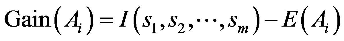
The attribute  with the highest information gain is chosen as the root node, the branches of the root node is formed according to various distinctive values of
 . The tree grows until if all the samples are all of the same class, and then the node becomes a leaf and is labeled with that class. From the tree, understandable rules can be extracted in a quick processing [17]. Here, the task of decision tree development is conducted using C4.5 classification algorithm where each tree leaf is allocated to a class of chemotherapy outcome along with number of misclassified cases.
2.3.2. Bayesian Networks
Generally, Bayesian classifiers are statistical approaches capable of predicting class membership likelihoods like the probability of the training set belonging to a specific class. It is based on Bayes theorem and well known for its high accuracy and speed when applied to a large data collection. Here, simple estimator Bayesian network has been used.
Let X be a sample whose class is to be defined and let H be a hypothesis that X belongs to class C. In this classification task,  needs to be defined which is the probability that the hypothesis H holds based on the data sample X. It can be calculated through:
 (9)
(9)
where  and
and  are the prior probability of H and X respectively.
  is the posterior probability of X given on the H. In model training these three values are calculated and the probability for sample X to be in hypothesis H can be determined. There are two essential features that define a Bayesian network: a directed cyclic graph in which each node denotes a random variable, either discrete or continuous values, as well as a set of conditional probability tables. Let
  be a data tuple related to the correspondent attributes
 . Given that every attribute is conditionally independent on its non-descendent and parents in the network, the following equation is a representation of joint probability distribution.
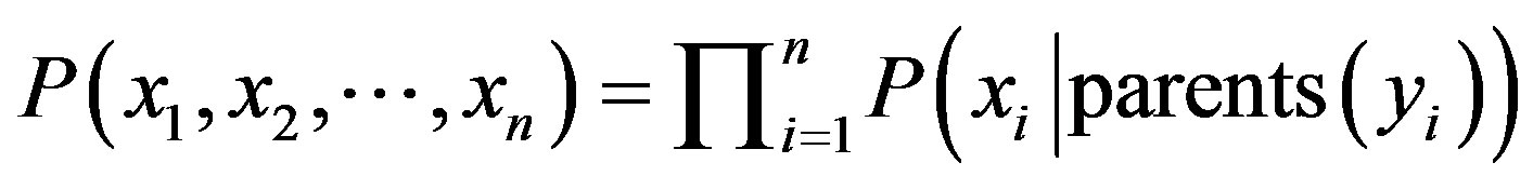 (10)
(10)
where the values for  are related to the entries for
 ;
;  is the probability of a specific combination of values of X. Probability distribution, with the probability of each class may be the output of this classification process [18].
2.3.3. Logistic Regression
Logistic regression is used primarily for predicting binary or multi-class dependent variables. This algorithm’s response variable is discrete and it builds the model to predict the odds of its occurrence. This method’s restrictive assumptions on normality and independence induced an increased application and popularity of machine learning techniques for real-world prediction problems. In this study, multinomial logistic regression is applied which is an algorithm that constructs a separating hyperplane between two sets of data by using the logistic function to express distance from the hyperplane as a probability of dichotomous class membership:
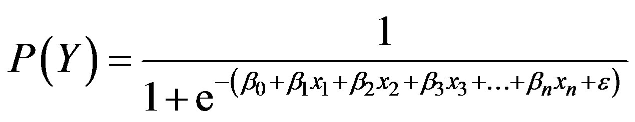 (11)
(11)
In this equation,  symbolizes discrete or continuous predictor variables with numeric values; in the case of depending variable (Y) being dichotomous, we use this algorithm. The constants
  are the regression coefficients estimated from training data which are typically computed by using an iterative maximum likelihood technique. Normally, this formula’s justification is that the log of the odds, a number that goes from
  to +
to + , is a linear function. Particularly by using this model, stepwise selection of the variables can be made and the related coefficients calculated. In producing the LR equation, the statistical significance of the variables used to be determined by the maximum-likelihood ratio [19].
2.3.4. Artificial Neural Networks
Artificial Neural Network (ANN) is biologically inspired analytical method which is able of modeling extremely complex non-linear functions. Here, a common architecture named multi-layer perceptron (MLP) with learning by back-propagation algorithm is built. A neural network is a compound of linked input/output units in which every link has an associated weight. Adjusting the weights is the core phase for predicting the correct class label of input through iterative learning. This method is popularly used in classification and prediction tasks with high tolerance to noise and the ability to classify unseen patterns [19]. Here, algorithm has conducted the learning process 500 times and the network structure is shown in a simple way when only two attributes have been applied as inputs. The structure of a two-input, one hidden layer neural network for our task with five outputs has been presented in Figure 2.
2.3.5. Radial Basis Function
A radial basis function network (RBFN) is an artificial intelligence network in which its activation function is simply radial basis in a linear combination. This type of network was designed to view a problem in curve-fitting (approximation) and high dimensional space. The real inspiration behind the RBF technique is finding amultidimensional function that offers the best fit to training tuple and then applies this multidimensional surface to interpolate the test data through regularization [20]. Gaus-

Figure 2. The simplified structure of applied neural network only with two of our attributes “HIV” and “recent TB infection”, one hidden layer and five classes in output layer. The structure is much simplified neural networks are popularly applied in classification and prediction, as they have advantages such as high tolerance to noise, and the ability to classify unseen patterns.
sian radial basis function is applied algorithm in this study.
2.3.6. Support Vector Machine
Support vector machine (SVM) is a new classification method for both linear and non-linear data. SVM applies nonlinear mapping to transform the original training tuple into a higher dimension. It seeks the optimal linear separation hyperplane which is the decision boundaries separating the tuple based on their class labels.Polykernel support vector machine has been applied in this investigation.Let the dataset Abe considered as ,
,  where
where  is the set of learning data with correspondent class label
 . For a two-class related training dataset, for instance, every
  can take either +1 or −1. This could also be generalized to n dimensions and the SVM duty is to find the best dividing lines that can be drawn and divide all of the tuples of every class from the others. For multidimensional classes the hyperplanes should be found asdecision boundaries. This can be arranged by defining the maximum marginal hyperplane (MMH) since models with larger hyperplane are more accurate at classification [18].
2.4. Accuracy Measurements
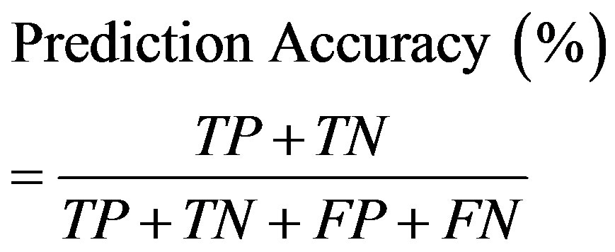
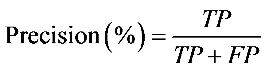
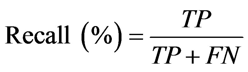
In order to evaluate the prediction rate, the following related parameters need to be measured. Prediction accuracy percentage (model Accuracy), model fitness, recall, Precision, F-measure, and ROC area are considered criteria used to assess the models’ validity. In confusion matrix (Figure 3) in which the columns denote the actual cases and the rows denote the predicted cases, the accuracy of model obtained from training set (model fitness) and testing set (prediction accuracy) are calculated. The prediction accuracy is the percentage of correct prediction (true positive + true negative) divided by the total number of predictions. In machine learning, sensitivity is simply termed recall (r) and precision is the positive predicted value. F-measure is a harmonic means of precision and recall and the higher value of it merely reveals the better performance of a prediction task.
Another comparative criterion is Roc curve which is a two-dimensional graph where the true positive (TP) rate on the Y axis is plotted on the false positive (FP) rate on the X axis [21].
 (12)
(12)
 (13)
(13)
 (14)
(14)
 (15)
(15)
 (16)
(16)
2.5. The Database
The available dataset has been driven from gathered records by health practitioners, nurses, and physicians at local TB control centres throughout Iran in 2005. In tuberculosis control centres, health deputies of each province in a network system collected data in every appointment. By using “Stop TB” software, more than 35 parameters were collected and through applying bivariate

Figure 3. A simple confusion matrix, a two-by-two table, values in the main diagonal (TP and TN) represent instances correctly classified, while the other cells represent instances incorrectly classified (FP and FN errors).
correlation method; those independent variables which are significantly correlated with target outcome are selected as predictors (P <= 0.05). They are presented and defined in Table 1. The distribution of corresponding outcomes of TB treatment course based on their frequency in training and testing sets are shown in Table 2. Due to normal and non-normal distribution variables which were tested by both Kolmogorov-Smirnov test and visual shape of attribute’s distribution, Pearson and Spearman rho methods were applied to find highly correlated factors.
3. Experiments and Results
3.1. Feature Selection
Significant Kolmogorov-Smirnov test confirmed with the shape of their distribution showed the distribution of our variables; Spearman rho was applied for those with nonnormal distribution.
Having considered the results, it is revealed that males are more likely to not get cure and complete the course of TB treatment (r = −0.082, P < 0.0001).
As patients get older there is more probability to get undesirable result from treatment course (r = 0.158, P < 0.0001).
The more under-weight the patients are, they are more likely at the risk of unwelcome outcome (r = −0.056, P < 0.0001).
TB cases with extra-pulmonary TB are more likely at the risk of outcomes like quitting, failing or death (r = −0.066, P < 0.0001).
There is 0.127 more probability that immigrants from Iraq, Pakistan, and Afghanistan to quit, get failed in treatment course (r = 0.127, P < 0.0001). TB patients who are living in abroad as well as mobile cases are −0.027% more possible to get undesirable outcome compared with
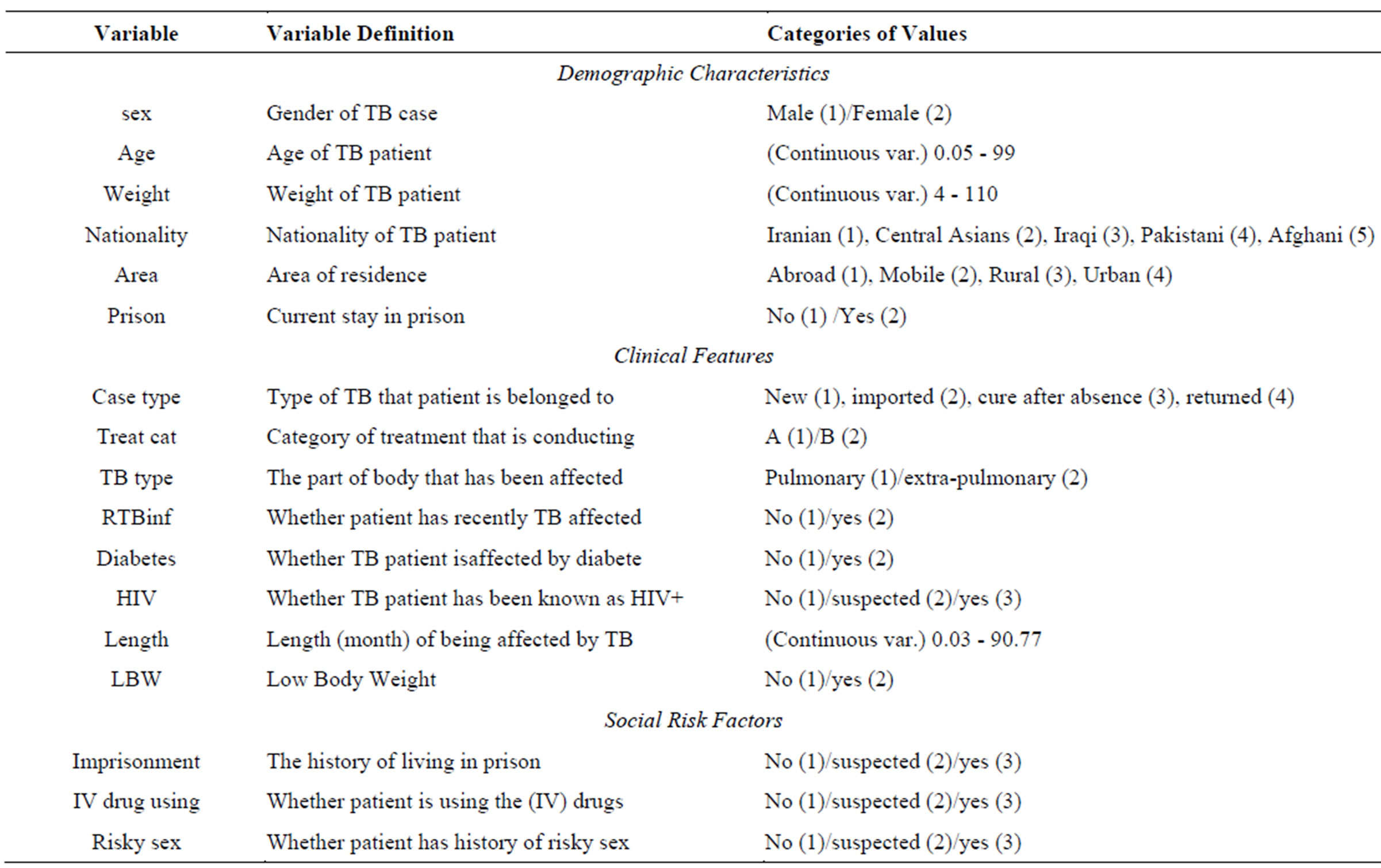
Table 1. Patients’ attributions applied for experiments, their definitions and their range of values.
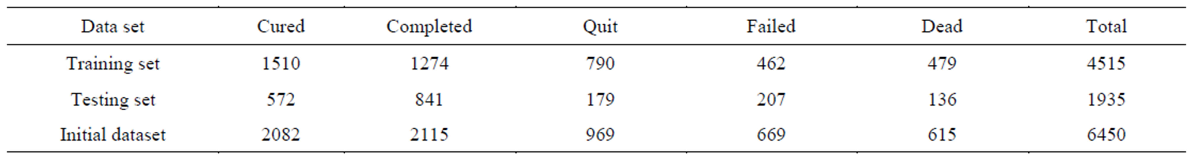
Table 2. The real outcomes happened for Tuberculosis patients for initial, training and testing sets with their corresponding outcomes.
those who are living in urban and rural areas (r = −0.027, P < 0.0001).
Prison residency and treatment outcome completion are significantly correlated (r = −0.026, P < 0.0001).
The more time TB patients spend affected with this infectious disease, there is 0.073 times more chance of non-desirable outcomes of tuberculosis treatment course.
Diabetic or HIV+ TB cases are positively prone to have worse result of treatment course (rho diabetes = 0.029, P < 0.001 & rho HIV = 0.045, P < 0.05).
Also, the probabilities of having imprisonment history in his/her life, consuming drugs through intravenous, or having unprotected sex increase the likelihood of unwanted outcome with r = 0.157, 0.0172, and 0.16 respectively (P < 0.000).
3.2. Classification Algorithms Analysis
In this work, six classifiers including DT, BN, LR, MLPRBF and SVM were applied to the patient dataset. Model development is conducted in two main steps including model fitness and model accuracy. To calculate the model fitness criteria we used the data of training set; however, to compute the model accuracy measurements, data of testing set is applied which is merely much more valuable to judge about our models accuracy. Related results of these experiments are demonstrated in Table 3.
Model fitness assessment by evaluating training accuracy is 84.45% for C4.5 decision trees; it is considerably less for Bayesian net where the value is 58.56%. The values of model fitness for logistic regression (56.5%), MLP (64.93%), RBF (50.65%), and SVM (53.04%) have been close. Having compared the Roc curves reveal that the area under curve for C4.5 has the most value for model fitness and accuracy with 0.96 and 0.97 respectively. This measurement is less for Bayesian net (0.85), logistic regression (0.82), MLP (0.81), RBF (0.79), and SVM (0.76) in terms of model accuracy. C4.5 decision tree has been able to build a model with greatest accuracy since the model fitness and prediction accuracy are 84.45% and 74.21% respectively.
Prediction accuracy for Bayesian networks has been calculated by 62.06%. Model accuracies obtained from other classifiers are different as this value for LR, MLP, RBF, and SVM have been 57.88%, 57.31%, 53.74%, and 51.36% respectively.
Figure 4 is the comparative Roc curves based on the given outcome of tuberculosis treatment including cure, complete, quit, failed or dead. This figure shows six Roc curves for six developed models based on the given outcome. For the outcome “cure”, C4.5 has outperformed than other classifiers with area under curve 0.958. Similarly, the most accurate result for outcomes ‘completed’ and “quit” obtained for C4.5 with 0.966 and 0.956 respectively. C4.5 has also performed the best for the outcome “failed” and “dead” by classifying 0.986 and 0.963 of cases correctly. Overall, these results of area under curve reveals better performance of C4.5 decision tree classification algorithm. Table 3 and Figure 4 present obtained results including model fitness and accuracy as well as produced area under ROC.