1. Introduction
It is well-known that, for the American option-pricing model, there is an optimal holding region for contracts holders (see [1-5]). The part of the boundary for the region is unknown (free boundary), which is often referred as the optimal excising boundary for option traders. This free boundary has to be calculated along with the option price of the security. The mathematical model for the problem is highly nonlinear and there is no explicit solution representation even when volatility and interest rate are assumed to be constants (see [4]). On the other hand, for the financial world as well as for the intrinsic interest itself, it is extremely important to find the location of the free boundary along with the option price of the security. Particularly, people would like to know how the price of a security changes near the option expiry time since it may change dramatically [6,7].
During the past few decades, there are many research papers concerning for various option-pricing models. There are several Monographs devoted to this topic (see, for examples, [1,3,4,8]). For the American option model as well as its generalization, the existence and uniqueness are studied by many researchers ( here just a few examples, [2,5,9-12]). A basic fact is that the American option-pricing model can be reformulated as a variational inequality of parabolic type. Hence, many known results about existence and uniqueness can be applied to the model. However, the disadvantage of the method is that there is no information about the free boundary. To overcome the shortcoming, several authors employed other methods to establish the existence and uniqueness for the problem (see [7,13-17]). Because of the practical importance, many researchers paid a special attention to the asymptotic behavior for the free boundary near the expiration time(see [6,18-25]). Moreover, various numerical computations for the location of free boundary are also carried out by many people (see, for examples, [14,25-28] and the references therein). More recently, some global property of the free boundary attracts some interest. The authors of [29,30] proved that the free boundary is convex if the volatility in the model is assumed to be a constant. However, this global property is not valid in the real financial market since the volatility depends on time and other economical factors. When the volatility depends on time and the security, the problem becomes much more challenging. In this paper we would like to study some global property of the free boundary. We want to find how the optimal exercising boundary changes when the volatility changes during the life-time of the option contract. This question is very important for structured products in the financial world.
We first recall the classical model for the American option-pricing model with one security or one type of asset. Let  be the option price for a security such as a stock with price
  at time
 . Then it is wellknown that
  satisfies the Black-Scholes equation with no dividend [31,32]:
 (1.1)
(1.1)
where  is the interest rate and
  represents the market volatility of the stock,
  is the region defined below.
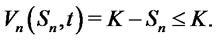
For the American put-option model (call-option is similar), in order to avoid loss for option holders, it is desirable to hold the option only when  lies in the region (called optimal holding region):
where  is the free boundary, which ensures
 , called the optimal exercising boundary.
On the free boundary , we know from the continuity of the option price that
  satisfies:
 (1.2)
(1.2)
 (1.3)
(1.3)
where  is the striking price.
We also know the payoff value at the terminal time  once the striking price is given:
 (1.4)
(1.4)
 (1.5)
(1.5)
For later use, we introduce :

where
In financial markets, the volatility  plays a major role for the option pricing model. Option price often changes dramatically when the stock market is in a chaotic movement. This was the case when the flash-crash happened on May 6, 2010 as well as the case on Oct. 19, 1987. On the other hand, for a relatively stable market, the volatility mainly depends on time. This is particularly true for an index fund such as S&P500 index in the U.S. market. Hence, we assume that
  throughout this paper. Our question is how the free boundary
  changes when the volatility
  changes during the life-span of the option contract. We show that there is a global comparison principle for the free boundary with respect to the change of volatility
 . Moreover, a global existence result is also established as a by-product. Our proof is based on the line method (see [15]), which is different from existing literature (see [21,13] and the references therein). Although the existence of a solution for the problem is already known, our method does have several advantages. One of them is that the free boundary is determined along with the option price at each discrete time simultaneously. Moreover, a global regularity for the free boundary is also obtained. To author’s knowledge, this regularity result is new and optimal (see [19, 21,12]).
The paper is organized as follows. In Section 2, we construct a sequence of approximation solutions by using the line method. After deriving some uniform estimates, a global existence is established. Moreover, an optimal global regularity for the free boundary is also obtained. In Section 3, we first derive some comparison properties for the approximation solution and then show that the limit solution preserves the same property. Some concluding remarks are given in Section 4.
Remark 1.1: After this paper is completed, the author learned that E. Ekströn proved a result in [33] (2004) about the monotonicity of option price with respect to volatility. However, there is no result about the comparison result for the free boundary. Moreover, the method in [33] is totally different from ours here. In addition, we also present a regularity result for the free boundary.
2. Existence and Uniqueness
Since our argument in Section 3 is based on the discrete problem, we give the complete details about the construction of the approximation solution sequence. We also show that the approximation sequence is convergent to the solution of the original problem (1.1)-(1.5). As a byproduct, an optimal regularity of the free boundary is obtained.
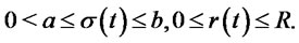
The following conditions are always assumed throughout this paper.
H(1): Let  for some
 . There exist positive constants
  and
and  such that
Now we construct an approximate solution sequence by using the line method.
Let  be a positive integer. Divide
  into
into 
subintervals with equal length :
:

Define

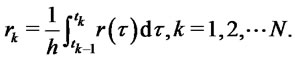
If we use difference quotient to approximate  and replace
  and
and  by
by  and
and , we have

This leads us to define the approximate solution  and
and  as follows:
From the terminal condition, we know

and . So we define

Suppose we have obtained  and
and , we can define
  and
and  as follows:
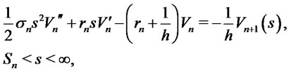 (2.1)
(2.1)
 (2.2)
(2.2)
 (2.3)
(2.3)
where we have extended  into the whole interval
  by
by

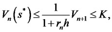
It is easy to see that the above free boundary problem (2.1)-(2.3) has a unique solution  for each
 . Actually, since the problem is one-dimensional one can find the solution
  and
and  explicitly (see [4] for detailed calculation).
Now we use the interpolation to define the free boundary  as follows:

Also, we define

We also use the notation


Our goal is to show that the approximate solution sequence  is convergent to the solution of the original free boundary problem (1.1)-(1.5).
To this end, we need to derive some uniform estimates.
Lemma 2.1: For all ,
,

Proof: From the definition, we see

if . Suppose we have shown that
  , we claim that
 . Indeed, if
  attains a negative minimum at some point
 , then at this minimum point, we see

which contradicts the right-hand side of the Equation (2.1). It follows that  on
on . By the definition of
  on
on , we see
  for
for . Consequently,
  on
on .
.
On the other hand, we claim that  has an upper bound
 . Indeed, it is obviously true for
 , which implies that
  when
when . We assume that
  is the first interval in which
 . Then, suppose that
  attains a positive maximum at an interior point
 , then at
 ,
, . Thus,

It follows from Equation (2.1) that
which is a contradiction. On the boundary ,
,
Obviously,  when
when . Consequently,
  in
in . Furthermore, from the boundary condition (2.2), we see
  for all
 .
.
Q.E.D.
Lemma 2.2: There exists a constant  such that

where  depends only on known data, but not on
 .
.
Proof: This estimate is similar to the energy estimate for a parabolic equation. Indeed, we introduce new variables:
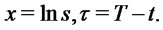
Define

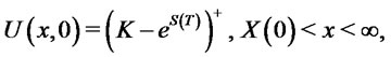
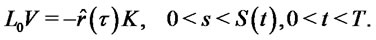
Then the original free boundary problem (1.1)-(1.5) is equivalent to the following one:
 (2.4)
(2.4)
 (2.5)
(2.5)
 (2.6)
(2.6)
 (2.7)
(2.7)
where


On the other hand, by the definition we know

It follows that
Thus,

Now we can extend  into the region
 , we use the continuity of
  and
and  in
in  to see that
  is a weak solution of the following problem:
 (2.8)
(2.8)
 (2.9)
(2.9)
where  if
if  and
and  if
if .
.
Now we can use the line method method to define  and
and  which are exactly the same as for a classical parabolic equation (see [34], estimate (5.15) on page 137) and obtain the desired energy estimate. By the definition, we see clearly that
  for
for .
.
Q.E.D.
Lemma 2.3: There exists a constant  such that

where  depends only on known data, but not on
 .
.
Proof: Note that  is uniformly Lipschitz continuous on
 . We may assume that
  is differentiable with a bounded derivative on
 .
.
Define

It follows that  satisfies the following equations:
 (2.10)
 (2.11)
 (2.12)
The maximum principle yields that  is uniformly bounded and the bound depends only on known data. By using the same argument, we can easily deduce the uniform bound for
 .
.
Q.E.D.
Let  be a small number and define

Lemma 2.4: There exists a constant  such that

where  depends only on the known data and
 , but not on
 .
.
Proof: From the theory of parabolic equations, we may assume that  is differentiable up to
 . Set
. Set

From the boundary condition (2.5), we see

It follows by (2.6) that

From the Equation (2.4) and the boundary conditions (2.5) and (2.6), we see

which is uniformly bounded.
By differentiating Equation (2.4) with respect to x twice, we see  satisfies

For any , the Schauder’s theory implies that
  is uniformly bounded and the bound depends on known data and
 . Now we can apply the maximum principle again on
  to conclude that
  is uniformly bounded. One can also use the same argument for
  to conclude the estimate for
  in
in . Similar estimates hold for the discretized solution
  and
and .
.
Q.E.D.
Lemma 2.5: There exists a constant  such that

where  depends only on known data and
 , but not on
 .
.
Proof: First of all,  is continuous and is also differentiable on
  except
 . It follows that
 .
.
From the definition of  and the boundary condition (2.2), we know that, for
 ,
,

Note that , then

It follows that

where  depends only on known data and
 .
.
Q.E.D.
With the results of Lemmas 2.1-2.5, we are ready to prove the following theorem.
Theorem 2.6: The free boundary problem (1.1)-(1.5) has a unique solution  with
with
 and
and .
.
Proof: First of all, the existence of a weak solution  in
in  follows the exactly same argument as that in [34] (Theorem 5.1, page 138). The uniqueness follows from the variational inequality. Moreover, regularity theory for parabolic equation implies that

Moreover, since the coefficients of the Equation (2.4) depends only on , we use the interior regularity of parabolic equations to conclude that
 .
.
To see the regularity of the free boundary, we use Lemma 2.5 to see  and
and

It follows that

Hence, by Ascoli-Arzela’s lemma, we can extract a subsequence, still denoted by , such that
  converges to a function, denoted by
 . Moreover,
 . Since
  is arbitrarily, we have
 .
.
Furthermore, since , we use
  - estimate to obtain that for any
 ,
,
where  depends only on known data,
  and
and .
.
Now we convert back to the original variables to conclude that

By Sobolev’s embedding, we know that  and
and  are continuous over
 . On the other hand, since
we obtain

To see more regularity for , we use the boundary condition (2.5)-(2.6). Indeed, from the condition (2.5)- (2.6), we see

We differentiate (2.6) to find
From the Equation (2.4) we obtain

It follows that

Now we consider the free boundary problem for  in
in :
:


It is easy to see that a unique solution  exists with
 . It follows that

Q.E.D.
Remark 2.1: For the existence and uniqueness, we only need to assume that  and
and  are of class
  with a positive lower bound for
 .
.
3. Properties of Free Boundary
As we mentioned in the introduction, we are interested in how the free boundary changes when  changes. It turns out that a comparison principle holds.
Theorem 3.1: Let  and
and  satisfy the assumption H(1). Let
  and
and
 be the solutions of the problem (1.1)- (1.5) corresponding to
  and
and .
.
If  on
on , then

To prove the theorem, we show that the comparison property holds for the discrete solution under certain condition.
Lemma 3.1: If , then

Proof: If necessary, we may use an approximation to replace  by a smooth convex function on
 . Without loss of generality, we may simply assume
 . Then from the regularity theory, we know that
  is differentiable in
 . Let
. Let

Now for , we differentiate the Equation (2.1) twice with respect to
  to see that
  satisfies the following equation:

From the maximum principle, we see that  can not attain a negative minimum if
 .
.
On the other hand, from the Equations (2.1) and (2.1) we see

It follows that, if ,
,

Once we know , we can use the maximum principle to obtain the same conclusion for
 . After a finite number of steps, we obtain the desired result of Lemma 3.1.
Q.E.D.
Since we are interested in the relation between  and
and , for convenience we use
 and
and  instead of
  and
and .
.
Lemma 3.2: For ,
,

Proof: Let

We differentiate Equation (2.1) for  with respect to
  to obtain:

From Lemma 3.1, we see that

The maximum principle implies that  can not attain a negative minimum at an interior point in
 .
.
On :
:

We differentiate  with respect to
  to obtain

It follows that  for
for  when
when . Now we can use the same argument to obtain the same conclusion for
 .
.
Moreover, from the second boundary condition, we have
 .
.
Also, from Equation (2.1) we know

It follows that

Since  attains its minimum 0 at the boundary
 , by Hopf’s lemma, we see
 . Thus,

Q.E.D.
Now we are ready to prove the main theorem in this section.
Proof of Theorem 3.1: Let  and
and  satisfy the assumption H(1). Let
  and
and  be the solutions of (1.1)-(1.5) corresponding
  and
and . If
. If  on
on . We define

Let  be the solution of the problem (2.1)- (2.3) corresponding to the volatility
 . It is clear that
  for
for  if
if  on
on
 . By Lemma 3.1 and Lemma 3.2, if
  we have

From the definition of , we know that

provided that .
.
Since  and
and  are uniformly convergent to
  and
and , respectively, as
 . It follows that

It is also clear that  on
on .
.
Q.E.D.
Remark 3.1: It is clear that the comparison result in Theorem 3.1 still holds if  with a positive lower and upper bounds.
4. Conclusion
When the volatility is a constant, it has been known for a long time that the option price is bigger when the volatility is bigger. However, when the volatility is a function of time,  , it is not clear how the option price nor the optimal excise boundary change when the volatility changes for the whole time period
 . In this paper we answered such a question. We show that a comparison property for option price and the optimal excising boundary hold (Theorem 3.1) when the volatility
 . This result is important for option traders. Moreover, we proved a global regularity result for the free boundary by using a very different method from the existing literature.
5. Acknowledgements
Some results in this paper were reported at the international conference “Problems and Challenges in Financial Engineering and Risk Management” held in Tongji University from June 23-24, 2011. The author would like to thank Professor Baojun Bian, Professor Xinfu Chen, Professor Min Dai, Professor Weian Zheng and other participants for their comments, which improves the original version of the paper.