Quasi-Degenerate Neutrino Masses with Normal and Inverted Hierarchy ()
1. Introduction
The presently available neutrino oscillation observational data [1-5] on two neutrino mass-squared differences ( ), is found to be insufficient to predict the three absolute neutrino masses in case of quasi-degenerate neutrino (QDN) mass models [6-14], as three independent equations are required for solving three unknown values of absolute neutrino masses. The values of the absolute neutrino mass scale ranging from 0.1 eV to 0.4 eV have been taken as input parameters in most of the theoretical calculations [6-15] in the literature. However, since the present tightest cosmological upper bound of the sum of three absolute neutrino masses, has gone down to the lowest value, ∑ mi ≤ 0.28 eV [16,17], a larger value of neutrino mass mi ≥ 0.1 eV in QDN models, has to be ruled out. Further the upper bound value of neutrino mass parameter mee ≤ 0.27 eV appeared in the neutrinoless double beta decay (0νββ) experiments [18], also disfavours larger values of neutrino mass eigenvalues with same CP-parity. Investigations on QDN models for both normal hierarchical (NH) and inverted hierarchical (IH) patterns of the three absolute neutrino masses, require detailed numerical analysis to check whether such QDN models can really accommodate lower values of absolute neutrino masses mi ≤ 0.09 eV which is consistent with the above cosmological bound. In addition, the solar mixing angle lying below the tri-bimaximal mixing (TBM) [19-21], which is consistent with present observational data [1-5] and the effects of CP-phases on three absolute neutrino masses, are also important ingredients for further analysis of QDN models. We address all these issues in the present work and show the validity of the quasi-degenerate models for lower values of neutrino masses mi ≤ 0.09 eV. This constitutes the main part of our work which differs from others on the mass scale rather than on the resulting lower solar mixing angles. We first introduce a general classification of QDN models based on their CP-parity patterns in the three absolute neutrino masses, and then parameterize the mass matrices using only two unknown parameters (ε, η) for achieving a practical numerical solution within µ – τ symmetry. Finally we present a detailed numerical analysis and results.
2. Parameterizations of Neutrino Mass Matrix
A general μ – τ symmetric neutrino mass matrix [22-24] with its four unknown independent matrix elements, requires at least four independent equations for a realistic numerical solution,
 (1)
(1)
The three mass eigenvalues mi and solar mixing angles θ12, are given by

 . (2)
. (2)
The observed mass-squared differences are then calculated as
 (3)
(3)
In the basis where charged lepton mass matrix is diagonal, we have the leptonic mixing matrix UPMNS = U of the form [23,24],
 (4)
(4)
The neutrino mass parameters mee appeared in the neutrinoless double beta decay (0νββ) and the sum of the three absolute neutrino masses in WMAP cosmological bound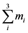 , are given respectively by,
 (5)
(5)
A general classification for the three types of quasidegenerate neutrino mass models [22] with respect to the Majorana CP-phases in their three mass eigenvalues, is adopted here. Diagonalisation of the left-handed Majorana neutrino mass matrix mLL in Equation (1) is given by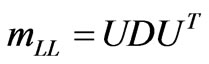 , where U is the diagonalising matrix in Equation (4) and
  is the diagonal matrix with two unknown Majorana phases
 . In the basis where charged lepton mass matrix is diagonal, the leptonic mixing matrix is given by
 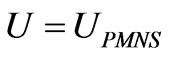 [23,24]. We then adopt the following classification according to their CP-parity patterns in the mass eigenvalues mi, namely, Type IA:
  for
for  ; Type IB:
  for
for  and Type IC:
  for
for  respectively. We now introduce the following parameterization of μ – τ symmetric neutrino mass matrices mLL which satisfy the above classifications [22].
3. Numerical Analysis and Results
We first estimate the numerical values of the three absolute neutrino masses. As discussed before, we need to introduce the neutrino mass scale m3 as input parameter in addition to the observational data [1-5] on solar and atmospheric neutrino mass-squared differences ( and
and ). For numerical analysis we use the best-fit values of the global neutrino oscillation observational data [1-5]
 eV2and
 eV2and also define the following parameters
 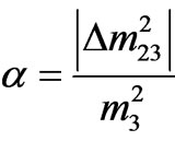 and
and , where m3 is the input quantity. For quasidegenerate model with normal hierarchy (NH-QD), the other two mass eigenvalues are estimated from,
 (6)
(6)
and for quasi-degenerate model with inverted hierarchy (IH-QD) the mass eigenvalues are extracted from,
 (7)
(7)
For suitable input value of m3, one can estimate the values of m1 and m2 for both NH-QD and IH-QD models, using the observational values of  and
and . Table 1 gives the calculated numerical values for both models.
In the next step we parameterize the mass matrix Equation (1) into three types: Type IA with
 : The mass matrix of this type [22, 25,26] can be parameterized using two parameters (ε, η):
 . (8)
. (8)
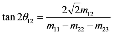
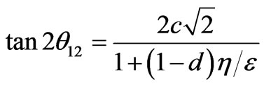
This predicts the solar mixing angle,
 . (9)
. (9)
When we choose the values c = d = 1.0, we get the tribimaximal mixings (TBM),  (which is
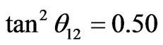 ) and the values of ε and η are calculated for both NH-QD and IH-QD models, by using the values of Table 1 in these two eigenvalue expressions: m1 = (2ε – 2η) m3 and m2 = (ε – 2η) m3. The results are given in Table 2 for
 . The solar angle can be further lowered by taking the values c < 1 and d > 1 while using the earlier values of ε and η extracted using TBM. For tan2θ12 = 0.45 case, the results are given in Table 3 Type IB with
 : This type [22,25, 26] of quasidegenerate mass pattern is given by the mass matrix,
 (10)
(10)
This predicts the solar mixing angle,
 , (11)
which gives the TBM solar mixing angle with the input values c = 1.0 and d = 1.0. Like in Type-IA, here ε and η values are computed for NH-QD and IH-QD, by using Table 1 in the corresponding two eigenvalue expressions: m1 = (1 – 2ε– 2η) m3 and m2 = (1 + ε – 2η) m3. Type IC with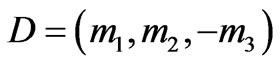 : It is not necessary to treat this model [22] separately as it is similar to Type-IB except

Table 1. The absolute neutrino masses in eV estimated from oscillation data [1] (Using calculated value of β = 0.03166).

Table 2. Prediction for tan2θ12 = 0.50.
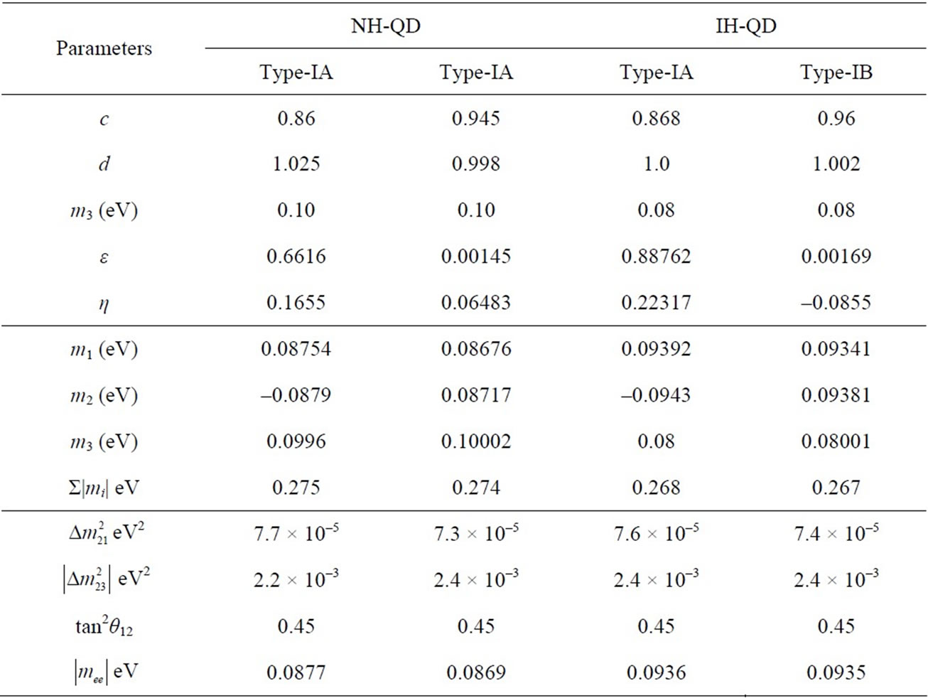
Table 3. Prediction for tan2θ12 = 0.45.
for the interchange of two matrix elements {22} and {23} in the mass matrix in Equation (10), and this effectively imparts an additional odd CP-parity on the third mass eigenvalue m3 in Type-IC. Such change does not alter the predictions of Type IB. A self explanatory results for two models of Types-IA and IB, for  and
and , are presented in Tables 2 and 3 respectively.
4. Conclusions
We have studied the effects of the Majorana phases on the prediction of absolute neutrino masses in three different types of QDN models having both normal and inverted hierarchical patterns within µ – τ symmetry. These predictions are consistent with observational data on the mass-squared difference derived from various neutrino oscillation experiments, and with the upper bound on absolute neutrino mass parameter in 0νββ decay as well as upper bound of  obtained from cosmological observations. It has been found that the QDN models with mi ≤ 0.09 eV, are still far from discrimination and hence not yet ruled out. The prediction on solar mixing angle is also found to be lower than TBM value viz,
  which coincides with the best-fit in the neutrino oscillation data [1]. The result shows the validity of NH-QD and IH-QD models. The results presented in this article are new and have important implications in the discrimination of neutrino mass models.
5. Acknowledgements
Ng. K. F. thanks the University Grants Commission, Government of India for sanctioning the project entitled “Neutrino masses and mixing angles in neutrino oscillations” vide Grant. No 32-64/2006 (SR). This work was carried out through this project.