A Generalization of Cramer’s Rule

Hugo Leiva^*

Department of Mathematics, Louisiana State University, Baton Rouge, LA, USA.

DOI: 10.4236/alamt.2015.54016                

Abstract

In this paper, we find two formulas for the solutions of the following linear equation , where is a real matrix. This system has been well studied since the 1970s. It is known and simple proven that there is a solution for all if, and only if, the rows of A are linearly independent, and the minimum norm solution is given by the Moore-Penrose inverse formula, which is often denoted by ; in this case, this solution is given by . Using this formula, Cramer’s Rule and Burgstahler’s Theorem (Theorem 2), we prove the following representation for this solution

, where are the row vectors of the matrix A. To the best of our knowledge and looking in to many Linear Algebra books, there is not formula for this solution depending on determinants. Of course, this formula coincides with the one given by Cramer’s Rule when .

Keywords

Linear Equation, Cramer’s Rule, Generalized Formula

Received 27 April 2014; accepted 4 December 2015; published 7 December 2015

1. Introduction

In this paper, we find a formula depending on determinants for the solutions of the following linear equation

(1)

or

(2)

Now, if we define the column vectors

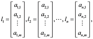
then the system (2) also can be written as follows:

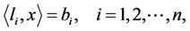(3)

where denotes the innerproduct in and A is real matrix. Usually, one can apply Gauss Elimination Method to find some solutions of this system, and this method is a systematic procedure for solving systems like (1); it is based on the idea of reducing the augmented matrix

(4)

to the form that is simple enough such that the system of equations can be solved by inspection. But, to my knowledge, in general there is not formula for the solutions of (1) in terms of determinants if.

When and, the system (1) admits only one solution given by, and from here one can deduce the well known Cramer Rule which says:

Theorem 1.1. (Cramer Rule 1704-1752) If A is matrix with, then the solution of the system (1) is given by the formula:

(5)

where is the matrix obtained by replacing the entries in the ith column of A by the entries in the matrix

A simple and interested generalization of Cramer Rule is done by Prof. Dr. Sylvan Burgstahler ( [1] ) from University of Minnesota, Duluth, where he taught for 20 years. This result is given by the following Theorem:

Theorem 1.2. (Burgstahler 1983) If the system of equations

(6)

has(unique) solution, then for all one has

. (7)

Using Moore-Penrose Inverse Formula and Cramer’s Rule, one can prove the following Theorem. But, for better understanding of the reader, we will include here a direct proof of it.

Theorem 1.3. For all, the system (1) is solvable if, and only if,

(8)

Moreover, one solution for this equation is given by the following formula:

(9)

where is the transpose of A (or the conjugate transpose of A in the complex case).

Also, this solution coincides with the Cramer formula when. In fact, this formula is given as follows:

(10)

where is the matrix obtained by replacing the entries in the jth column of by the entries in the matrix

In addition, this solution has minimum norm, i.e.,

(11)

and.

The main results of this work are the following Theorems.

Theorem 1.4. The solutions of (1)-(3) given by (9) can be written as follows:

(12)

Theorem 1.5. The system (1) is solvable for each, if, and only if, the set of vectors formed by the rows of the matrix A is lineally independent in.

Moreover, a solution for the system (1) is given by the following formula:

(13)

(14)

where the set of vectors is obtain by the Gram-Schmidt process and the numbers are given by

(15)

and.

2. Proof of the Main Theorems

In this section we shall prove Theorems 1.3, 1.4, 1.5 and more. To this end, we shall denote by the Euclidian innerproduct in and the associated norm by. Also, we shall use some ideas from [2] and the following result from [3] , pp 55.

Lemma 2.1. Let W and Z be Hilbert space, and the adjoint operator, then the following statements holds,

[(i)] such that

[(ii)].

We will include here a direct proof of Theorem 1.3 just for better understanding of the reader.

Proof of Theorem 1.3. The matrix A may also viewed as a linear operator; therefore and its adjoint operator is the transpose of A and.

Then, system (1) is solvable for all if, and only if, the operator A is surjective. Hence, from the Lemma 2.1 there exists such that

Therefore,

This implies that is one to one. Since is a matrix, then.

Suppose now that. Then exists and given we can see that is a solution of.

Now, since is the only solution of the equation

then from Theorem 1.1 (Cramer Rule) we obtain that:

where is the matrix obtained by replacing the entries in the ith column of by the entries in the matrix

Then, the solution of (1) can be written as follows

Now, we shall see that this solution has minimum norm. In fact, consider w in such that and

On the other hand,

Hence,.

Therefore, , and if.

Proof of Theorem 1.5. Suppose the system is solvable for all. Now, assume the existence of real numbers such that

Then, there exists such that

.

In other words,

Hence,

So,

Therefore, , which prove the independence of.

Now, suppose that the set is linearly independent in. Using the Gram-Schmidt process we can find a set of orthogonal vectors in given by the formula:

. (16)

Then, system (1) will be equivalent to the following system:

, (17)

where

. (18)

If we denote the vectors’s by

and the matrix by

then, applying Theorem 1.3 we obtain that system (17) has solution for all if, and only if, . But,

.

So,

From here and using the formula (9) we complete the proof of this Theorem.

Examples and Particular Cases

In this section we shall consider some particular cases and examples to illustrate the results of this work.

Example 2.1. Consider the following particular case of system (1)

(19)

In this case and. Then, if we define the column vector

Then, and

Therefore, a solution of the system (19) is given by:

(20)

Example 2.2. Consider the following particular case of system (1)

(21)

In this case and

Then, if we define the column vectors

then

Hence, from the formula (10) we obtain that:

.

Therefore, a solution of the system (21) is given by:

(22)

(23)

(24)

. (25)

Now, we shall apply the foregoing formula or (12) to find the solution of the following system

. (26)

If we define the column vectors

then and, , and.

Example 2.3. Consider the following general case of system (1)

. (27)

Then, if is an orthogonal set in, we get

and the solution of the system (1) is very simple and given by:

(28)

Now, we shall apply the formula (28) or (12) to find solution of the following system:

. (29)

If we define the column vectors

Then, is an orthogonal set in and the solution of this system is given by:, , and.

3. Variational Method to Obtain Solutions

Theorems 1.3, 1.4 and 1.5 give a formula for one solution of the system (1) which has minimum norma. But it is not the only way allowing to build solutions of this equation. Next, we shall present a variational method to obtain solutions of (1) as a minimum of the quadratic functional,

(30)

Proposition 3.1. For a given the Equation (1) has a solution if, and only if,

(31)

It is easy to see that (31) is in fact an optimality condition for the critical points of the quadratic functional j define above.

Lemma 3.1. Suppose the quadratic functional j has a minimizer. Then,

(32)

is a solution of (1).

Proof. First, we observe that j has the following form:

Then, if is a point where j achieves its minimum value, we obtain that:

So, and is a solution of (1).

Remark 3.1. Under the condition of Theorem 1.3, the solution given by the formulas (32) and (9) coincide.

Theorem 3.1. The system (1) is solvable if, and only if, the quadratic functional j defined by (30) has a minimum for all.

Proof. Suppose (8) is solvable. Then, the matrix A viewed as an operator from to is surjective. Hence, from Lemma 2.1. there exists such that

Then,

Therefore,

Consequently, j is coercive and the existence of a minimum is ensured.

The other way of the proof follows as in proposition 3.1.

Now, we shall consider an example where Theorems 1.3, 1.4 and 1.5 can not be applied, but proposition 3.1 does.

Example 3.1. It considers the system with linearly independent rows

.

In this case and

Then

Therefore, the critical points of the quadratic functional j given by (30) satisfy the equation:

i.e.,

.

So, there are infinitely many critical points given by

Hence, a solution of the system is given by

.

Conflicts of Interest

The authors declare no conflicts of interest.

References

[1]	Burgstahier, S. (1983) A Generalization of Cramer’s Rulle. The Two-Year College Mathematics Journal, 14, 203-205. http://dx.doi.org/10.2307/3027088
[2]	Iturriaga, E. and Leiva, H. (2007) A Necessary and Sufficient Conditions for the Controllability of Linear System in Hilbert Spaces and Applications. IMA Journal Mathematical and Information, 25, 269-280. http://dx.doi.org/10.1093/imamci/dnm017
[3]	Curtain, R.F. and Pritchard, A.J. (1978) Infinite Dimensional Linear Systems. Lecture Notes in Control and Information Sciences, Vol. 8, Springer Verlag, Berlin.