Bayesian Estimation of Non-Gaussian Stochastic Volatility Models ()
Keywords:Non-Gaussian Distribution; Stochastic Volatility; Laplace Density; Fat Tails; Kullback Leiber Divengence; Bayesian Analysis; MCMC Algorithm
1. Introduction
The Stochastic Volatility models have been widely used to model a changing variance of time series Financial data [1,2]. These models usually assume Gaussian distribution for asset returns conditional on the latent volatility. However, it has been pointed out in many empirical studies that daily asset returns have heavier tails than those of normal distribution. To account for heavy tails observed in returns series, [3] proposes a SV model with student-t-errors. This density, although considered as the most popular basic model to account for heavier tailed returns, has been found insufficient to express the tail fatness of returns.
[4] fitted a student-t-distribution and a Generalized Error Distribution (GED) as well as a normal distribution to the error distribution in the SV model by using the simulated maximum likelihood method developed by [5,6]. [7] considered a mixture of normal distribution as the error distribution in the SV model. He used a bayesian method via MCMC technique to estimate the model’s parameters. According to Bayes factors, he found that the t-distribution fits the Tokyo Index Return better than the normal, the GED and the normal mixture. However the mixture of normal distributions gives a better fit to the Yen/Dollar exchange rate than other models.
This survey of literature proves that we can’t affirm absolutely that one distribution is better than another one. The selection of a density should be based on other parameters. In our work, we consider a general model of nonGaussian centered error distribution. We prove that the efficiency of a specification of SV model depends on the dispersion of the data base. In fact, we find that when the data base is very dispersed, the Gaussian specification behaves better than the non-Gaussian one. On the contrary, if the data base presents a little dispersion measure, the non-Gaussian centered error specification will behave better than the Gaussian one. For this reason, we propose a general SV model where the diffusion of the stock return follows a non-Gaussian distribution.
Since it is not easy to derive the exact likelihood function in the framework of SV models, many methods are proposed in the literature to estimate these models. The four major approaches are: 1) the Bayesian Markov Chain Monte Carlo (MCMC) technique suggested by [8], 2) the efficient method of moments EMM proposed by [9], 3) the Monte Carlo likelihood MCL method developed by [10], and 4) the efficient importance sampling EIS method of [11]. In this work, we consider the MCMC method for the estimation of the model’s parameters.
The rest of the paper is organized as follow: in the second section, we present, in a comparative setting, the usual Gaussian and the general non-Gaussian SV models. Bayesian parameter estimator’s and the MCMC algorithm are described in the third section. The fourth section develops an application of a non-Gaussian centered error density. In particular, we consider the Laplace density as an example of non-Gaussian distribution for the data base that we have studied. We conclude in the last section.
2. Stochastic Volatility Model with Gaussian/Non-Gaussian Noise
As any nature field, Finance has adopted a simple model, developed over the years, that attempts to describe the behaviour of random time fluctuation in the prices of stocks observed in the markets. This model assumes that the fluctuation of the stock prices follow a log-normal probability distribution function. The simple log-normal assumption would predict a Gaussian distribution for the returns with variance growing linearly with the time lag. What is actually found is that the probability distribution for high frequency data usually deviates from normality presenting heavy tails.
In this section, we present the classical Gaussian SV model and we introduce a non-Gaussian centered error distribution as an extension to the SV models.
2.1. Gaussian Stochastic Volatility Model
The log Stochastic Volatility model is composed of a latent volatility equation and an observed return equation
 (1)
(1)
where  and
and  are two independent Wiener motions. The parameter
  is the mean reversion of the volatility equation,
  represents the expected of the Log volatility and
  is interpreted as the dispersion measure of the volatility.
According to the Euler discretization schema, we get
 (2)
(2)
where  and
and  follow the bivariate centered Normal distribution
  with the identity matrix
  of covariance. Here, the new parameters
  and
and  are related in deterministic way to
  and
and ,
,  and
and . The parameter
  represents the persistence of the volatility process,
  is its expected value and
  can be interpreted as the volatility of the volatility. Note that the errors
  and
and  are uncorrelated.
In order to consider a more general case of SV model, we propose in the next section, a non-Gaussian centered error distribution for .
.
2.2. Non-Gaussian Stochastic Volatility Model
We consider a Stochastic Volatility model with a non-Gaussian noise where the return  follows a nonGaussian distribution with a mean equal zero and a variance governed by stochastic effects. The proposed model is given by:
 (3)
(3)
The innovation term in the return equation  follows a Non-Gaussian centered distribution with the mean zero and the variance equal
 . The most popular non-Gaussian centered error distributions that has been applied in SV models are: Student distribution [3], Generalized Error Distribution [4], Mixture of Normal distribution [7],
  -stable distribution [12], Laplace distribution, Uniform distribution....Among these nonGaussian centered error density, we have chosen the Laplace one for being applied to SV model. We estimate the model’s parameters and we apply it to tha CAC 40 index returns data.
3. Bayesian Estimation of Non-Gaussian Stochastic Volatility Model
A long standing difficulty for applications based on SV models was that the models were hard to estimate efficiently due to the latency of the volatility state variable. The task is to carry out inference based on a sequence of returns  from which we will attempt to learn about
 , the parameters of the SV model. [13] uses the method of moments to calibrate the discrete time SV models. [14] improves the inference as they exploit the generalized method of moments procedure (GMM). The Kalman filter was used by [15].
Recently, simulation based on inference was developed and applied to SV models. Two approaches were brought forward. The first was the application of Markov Chain Monte Carlo (MCMC) technique; ([8,16-18]). The second was the development of indirect inference or the so-colled Efficient Method of Moments; ([19-21]).
In our paper, we have chosen the bayesian MCMC approach for the estimation of the parameter’s and the volatility vector.
For the non-Gaussian SV model, we define the parameter set  and the state vector
 .
.
We can obtain the joint distribution  from
from  and
and . Bayes rule states that the posterior distribution can be factorized into its constituent components:

where  is the likelihood function,
  is the distribution of the state variables, and
  is the distribution of the parameters, commonly called the prior.
[17] assume conjugate priors for the parameters  following Normal distribution
  and
and  following an Inverse Gamma distribution
  which implies that the posteriors densities for the parameters are proportional to
 (4)
(4)
where
 (5)
(5)
For , we have that
 (6)
(6)
With these posterior densities, the Gibbs sampler is applied and we get a Markov Chain for each parameter and thus the parameter’s estimator. The only difficult step arises in updating the volatility states. According to [8] the full joint posterior for the volatility is
 (7)
(7)
where

as a function of , the conditional variance posterior is quite complicated (we can’t simulate directly from this density)
 (8)
(8)
where
 and
and 
The simulation of the posterior density of the parameters requires the application of the Gibbs Sampler. However, we prove explicit expression for the simulated parameters. In fact, after some simple calculations applied to the posterior density, we find the following expression for the iterated parameters by the Bayesian method in the  iteration
 (9)
(9)
For the second parameter , with the same method, we can prove that:
 (10)
(10)
For the parameter , the volatility of volatility, the prior density is an Inverse Gamma
  with parameters
 , the expression of the estimators of this parameter is
 (11)
(11)
We have considered some statistical model distributions characterized by different density for the noise terms. For each density listed in the second section (Student, Laplace, Uniform), we can formulate one particular specification for SV model. We have conducted a Chi-deux test to select (among these three densities) the appropriate error distribution to our data base. The results indicate that the Laplace density is the suitable distribution compared to the student and the uniform ones. In the second step, we will take the Laplace SV model such as a particular case of non-Gaussian SV model to be compared to the standard Gaussian distribution model that is the Normal one. The next section will present the application study.
3.1. Application
In this section, we consider one particular case of non-Gaussian SV model that is the Laplace one. In fact, the application of the Chi-deux test has proved that this model is the more appropriate to our data base.
The study of this density is very interesting. In fact, Laplace density has been often used for modeling phenomena with heavier than normal tails for growth rates of diverse processes such as annual gross domestic product [22], stock prices [23], interest or foreign currency exchange rates [24,25], and other processes [26]. However, the Laplace density is not yet explored in the context of Stochastic Volatility model.
The Laplace SV model is defined as:
 (12)
(12)
The innovation term in the return equation ,
, .
.
The probability density function of a Laplace density is expressed as:
 .
.
In order to prove the efficiency of the Laplace model, we conduct a simulation analysis.
Simulation Analysis
This section illustrates our estimation procedure using the simulated data. We generate 1000 observations from the Stochastic Volatility Laplace (SVL) model given by equation (3.12), with true parameters ,
,  ,
, . True parameters are chosen arbitrary. The following prior distributions are assumed
 ,
,  ,
,  , (where IG represent the Inverse Gamma density).
We draw 6000 posterior samples of MCMC run. We discard the initial  samples as burn in period. Table 1 gives the parameter’s estimates for posterior means and standard deviation. Comparison of the Mean Squared Errors calculated with the Normal Stochastic Volatility model are larger than those calculated with the Laplace Stochastic Volatility model. This result proves that the Laplace Stochastic Volatility model better fits the model’s parameters and state variables.
The second step in our simulation study consists of testing the hypothesis that the choice of a specification is based on the dispersion measure of the data base. So, we simulate data bases with different variances. Results prove that when the data base is characterized by a little dispersion measure, the Laplace SV model performs a better specification for the parameters. In fact, the calculation of the Mean Squared Errors for the Laplace and the Normal model prove that this measure is greater for the Gaussian model. So, we should consider the estimators deduced from the Laplace (non-Gaussian) specification.
On the contrary, when the data base is very dispersed, it has been proved that the Gaussian SV model offers more precise estimation for the parameters.
From this simulation study, we can conclude that the selection of a model specification depends on data base characteristics. If we reject the normality assumption for a data base, we can accept it for another one.

Table 1. Simulation results for the Laplace and the Normal models.
Notes: 1. This table provides a summary of the simulation results for the Laplace and the Normal model. 1000 observations were simulated off the true parameters. We report in the third and the fourth column the average (mean(1)) and the standard deviation (Stdev.(1)) of each parameter calculated with 6000 simulated path. After discarding a burn in period of 2000 iterations, we compute the mean (mean(2)), the standard deviation (Stdev.(2)) and the mean squared error for each parameter. Results are presented in the three last columns. We present the confidence interval between brackets. 2. MSE for a parameter  is calculated with the following formula:
3.2. Empirical Application
After approving our methodology using simulated data, we apply our MCMC estimation method to daily stock returns data. On our work, we focus on the study of the French stock market index: the CAC40 index returns. The sample size is 5240 observations. The log difference returns are computed as ; where
  is the closing price on day
 .
.
Table 2 summarizes the descriptive statistics of the returns data. The series reveal negative skewness proving the asymmetry of the return distribution. The Kurtosis equal 24.86. The series present a large Kurtosis . So we reject the normality assumption. This conclusion is also verified by statistical test of normality.
Figure 1 shows the data histogram, the Normal and the Laplace one. It appears very clear that the distribution of our database is very close to the Laplace distribution, especially in the tails. In fact, when the Normal density ignores the queue observations, Laplace histogram represents these points so, the later density is more representative to our data then the former one.
In Table 3, we present the KL divergence that calculates the distance between the true (empirical) and the estimated distribution (Laplace, Normal). When the value of this criterion is large, the estimated distribution differs significatively from the true distribution. On the contrary, when this measure is small, we affirm that the estimated distribution is similar to the true one. For our data base, the KL divergence equals 0.0656 between data density and Laplace density. It equals 1.1653 between data density and Normal density. This proves that the non-Gaussian specification is more accurate to the data considered than the standard Gaussian specification.
3.3. Estimation Results
In the last section, we have rejected the Gaussian assumption for the return series of the CAC40 index.
Table 2. Summary statistics for daily return data on the CAC40 from January 2, 1987 to November 30, 2007.
Note: This table provides summary statistics for daily return data on the CAC40 French Stoch Exchange index from January 2, 1987 to November 30, 2007.
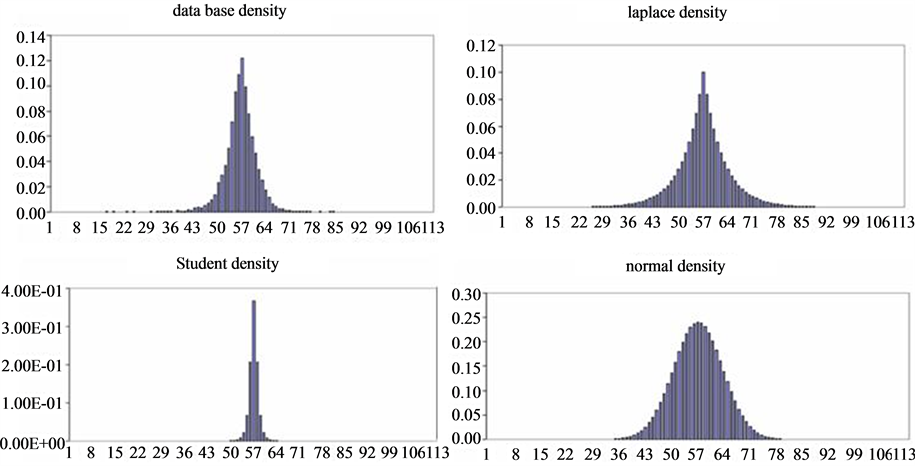
Figure 1. Database, Laplace, student and normal histogram. Note: The histograms of this figure are obtained with Microsoft excel program. For the first histogram, that represents the database density, we have classified our observation by class, we have computed the frequency in each class and the probability of each observation, and then we have represented the histogram. For the Laplace, Student and Normal density, we have generated. With Matlab, random vectors that follow each distribution with parameters (mean, variance) of the true database. Then, we compute the frequency and the probability of each observation and we represent the histogram with Microsoft excel.
Therefore, we have proven that the Laplace density is more consistent to our data base. In this section, we will apply the Laplace stochastic volatility model, that we have introduced in Equation (12), to the analysis of the CAC40 index returns. The number of MCMC iterations is 10000 and the initial 2000 samples are discarded. Table 4 reports the estimation results: the posterior means, standard deviations, and the Mean Squared Errors for CAC40 data.
The estimates of the volatility parameters  are consistent with the results of the previous literature. The posterior mean of
  is close to one, which indicates the well known high persistence of volatility on asset returns. Table 4 presents, also, the MSE calculated for each parameter for the Laplace and the Normal model. It seems clear that the Laplace model generates the little errors, except for the
  parameter. This result supports the choice of the non-Gaussian Stochastic Volatility model relatively to the Gaussian one.
In order to test the ability of the Laplace model to predict future returns, we perform an out of sample analysis. We consider 4000 observations for the inference of parameters. We simulate (5240 - 4000) artificial observations from the Laplace model and the Normal one. We compare each simulated vector of returns with the remainder observations.
In Table 5, we present the MSE found between the true observation vector and the returns generated with the Normal model in the third column. The second column shows the MSE calculated between true observations and returns vectors generated with the Laplace model. It seems clear that the Laplace model predict returns more accurately than the Normal one. In fact, the MSE obtained with the Laplace model is smaller than that obtained with the Normal model. The Laplace SV model generates a Mean Squared Error less than the errors generated
Table 3 . Kullback leiber divergence.
Note: This table summarizes the Kullback Leiber Divergence calculated between the true density and the estimated density: non-Gaussian (Laplace) in the second row, Gaussian (Normal) in the last row.
Table 4. Parameter estimates for the CAC40 index return data.
Note: Parameter estimates for the CAC40 index data from January 2, 1987 to November 30, 2007. For each parameter, we report the mean of the posterior density, the standard deviation of the posterior in parentheses and the MSE. Estimation for the Laplace SV model are presented in the second column. Results for the Normal model are given in the third column. The last row gives the MSE calculated for the whole model. The first number represents the MSE between estimated returns through Laplace model and the observed returns. The second number represents the MSE for estimated returns with the normal model and observed returns.
Table 5. Mean squared errors for the out of sample analysis.
Notes:1. In this table we present the out of sample analysis results. We take the first 4000 empirical observations to infer the parameter estimates for the Laplace SV model and the Normal SV model. We generate (5240 - 4000) artificial observations with the two model and we calculate the MSE between observed remainder returns and the simulated vector of return with Laplace model and with Normal model. 2. MSE for returns vector is calculated with the following formula: .
.
by the Normal SV model. This result indicates that the Laplace model (non-Gaussian) is able to predict returns better than the Normal one or the standard Gaussian one.
4. Conclusions
In this paper, we have considered the inference of SV model with non-Gaussian noise. By applying a Chi-deux test, we have chosen the suitable non-Gaussian distribution error for the data base considered in our study among different non-Gaussian distribution that has been considered in last studies (such as: Student, Uniform, Mixture of Normal,  -stable, ...). The Laplace SV model has been studied against the classical Gaussian SV model. After the simulation analysis, we have concluded that the selection of a model specification in favor of another depends on characteristics of data base. In fact, when data present little dispersion, non-Gaussian specification provides better estimation for the model parameters. On the contrary, when the dispersion of the data is very large, the standard gaussian specification is retained.
We have performed MCMC technique for the stochastic volatility model when returns follow a Laplace distribution allowing for an important characteristics of returns dynamic: Heavy tails or leptokurticity.
An application to daily CAC40 index returns over the years (1987-2007) illustrates the ability of the Laplace model to deal with heavy tails better than the Log-Normal model. An out of sample analysis proves that the Laplace model better predicts future returns. These results have been reached according to the calculation of the Mean Squared Error calculated between estimated parameters and true parameters.