Dynamics of a Hyperparasitic System with Prolonged Diapause for Host* ()
1. Introduction
Hosts and parasitoids are mostly univoltine and have no overlap between successive generations. Therefore, their interactions can be modeled by discrete differences. An early work by Beddington et al. [1] showed that discrete host-parasitoid models can produce a richer set of dynamic patterns than those observed in continuous-time models. More recently, many researchers [2-12] have reported that discrete host-parasitoid models can have very complex dynamics.
However, few studies have explored hyperparasitic systems using mathematical approaches and difference equations. Actually, hyperparasite can play a crucial role in the control of a host-parasitoid interaction if they are successfully established in the community. Furthermore, few works on complex dynamics in parasitic system have considered diapause. In the natural world, many insects which inhabit unpredictable environments display diapause for one year or more, which can be described as prolonged or extra-long diapause [13]. As observed in numerous laboratory and field experiments, diapause is induced by changing responses to temperature, photoperiod, humidity, hormonal treatment and other factors [14- 16]. Thus, incorporating hyperparasite and diapause in parasitic system is more realistic and more practical significance.
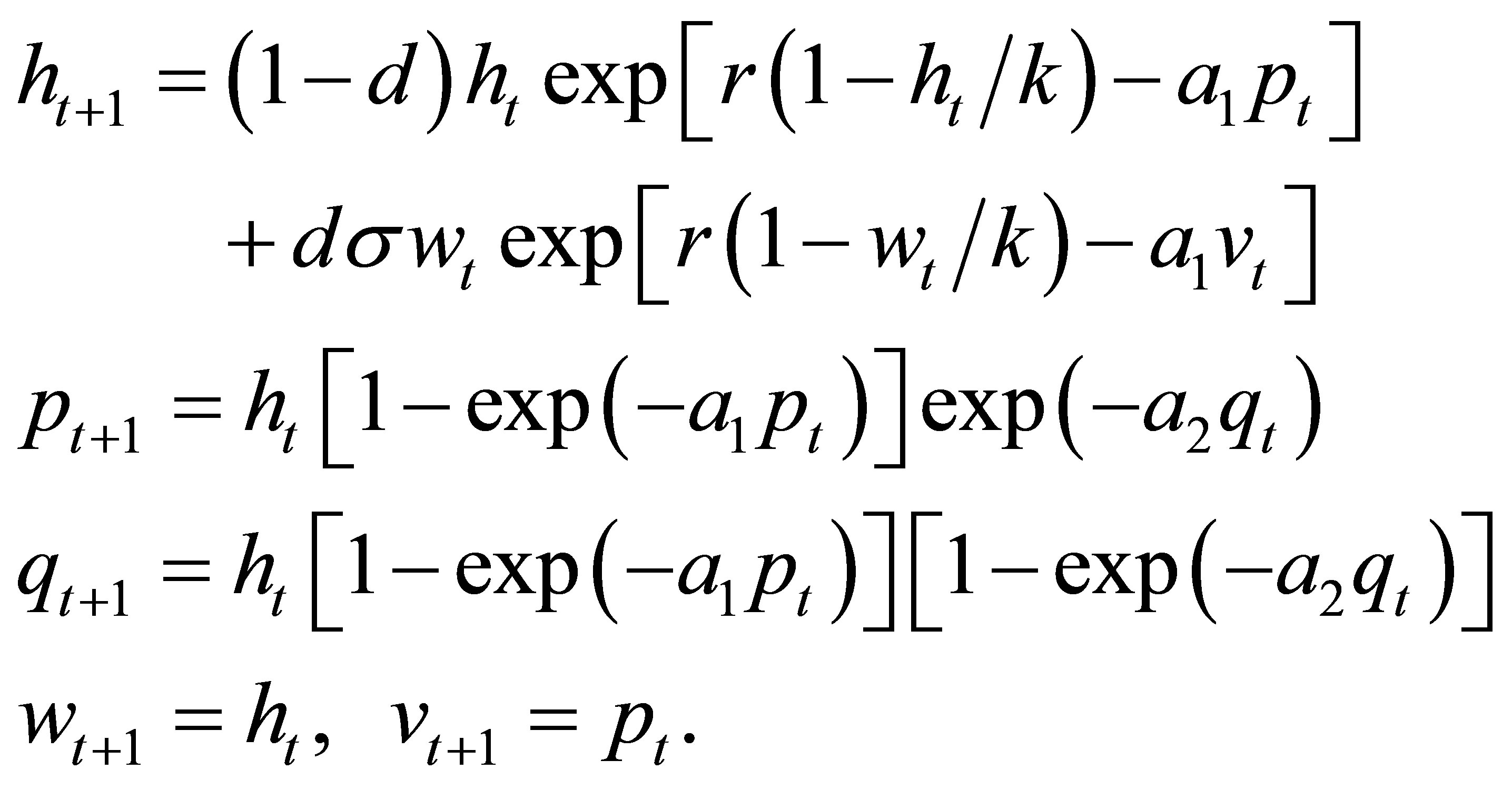
In the paper, a hyperparasitic system with prolonged diapause for host is investigated. In the system, we assume that host prolonged diapause occur at larval stage, and parasitoid attack is limited to egg stage before the initiation of host diapause. The parasitoids are physiological “regulators” [17]. In this case, the parasitoid can potentially attack all hosts, but do not undergo prolonged diapause itself. Such behavior has been reported for many ichneumons [18]. Hyperparasite only attacks the parasitoids that parasitize the hosts [19]. Based on the above considerations, the model can be represented by the following difference equation:
 , (1)
, (1)
where  denote the densities of the host, parasitoid, hyperparasite respectively at generation
 . In the absence of parasitism, the host adapts to Moran-Ricker model [20,21], that is to say
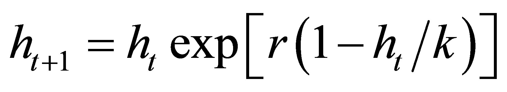 , where
  is the intrinsic growth rate and
  is the carrying capacity. The function
  given by Poisson distribution proposed by Nicholson and Bailey [22] stands for the probability that a host escapes parasitism,where
  is the parasitoid searching efficiency. By analogy with the above, the probability that a parasitoid escapes hyperparasites is
 . Accordingly,
  is the hyperparasite searching efficiency. The parameters
  and
and  represent diapause rate and survival rate of the host, respectively. According to their biological meaning,
  and
and  are non-negative and less than 1.
2. Stability Analysis
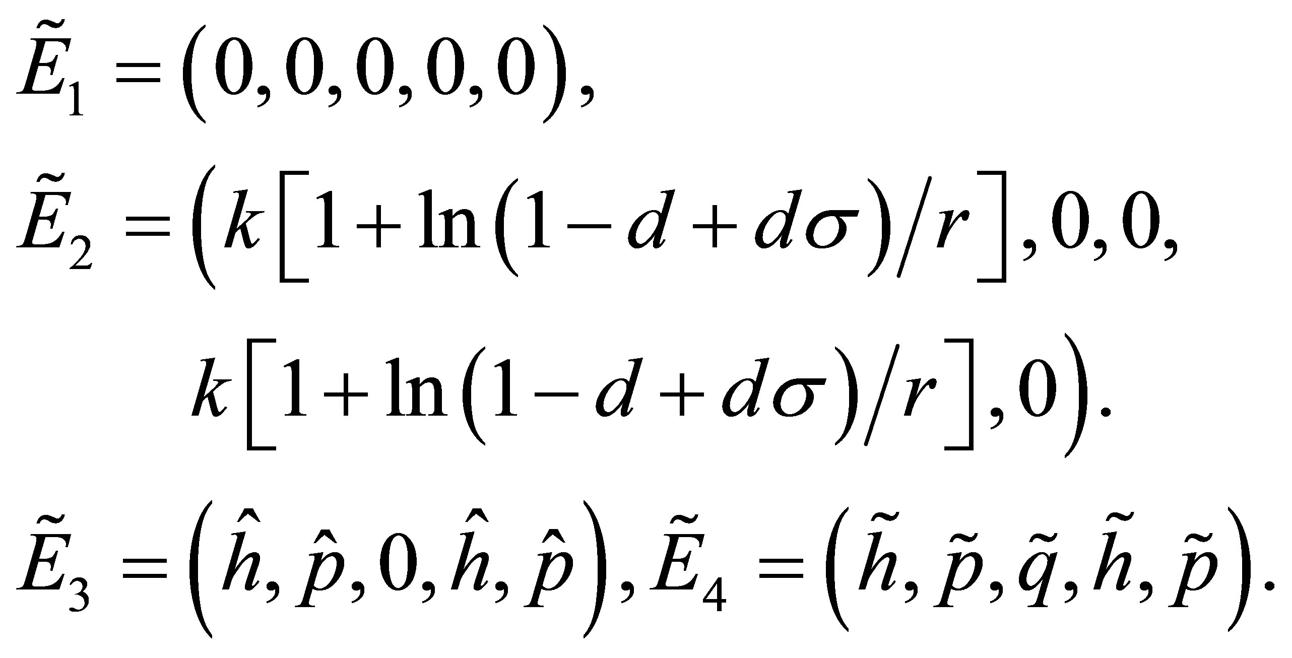
In this section, the existence and asymptotic stability analysis of the non-negative equilibrium points of system (1) are investigated. The system has four non-negative equilibrium points which are given by the following statements:
a) The equilibrium point  always exists.
b) The positive equilibrium point  is given by
  which exists if and only if
 (2)
(2)
The positive equilibrium point 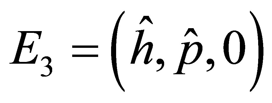 is given by
 (3)
(3)
which exists if and only if
 (4)
(4)
The positive equilibrium point  is given by
 (5)
(5)
which exists if and only if
 (6)
(6)
Analysis of the stability of the system (1) close to the above equilibrium points requires that the system is fully specified in terms of densities at time  and
and . For this, we introduce two variables,
  and
and , corresponding to the densities of hosts and parasitoids at time
  respectively. Then the system (1) corresponds to the following form:
 (7)
(7)
Accordingly, the four equilibrium points of the system (1) corresponds to the following forms respectively:
The stabilities of equilibrium points ,
,  ,
,  and
and  are as the same as these points

 and
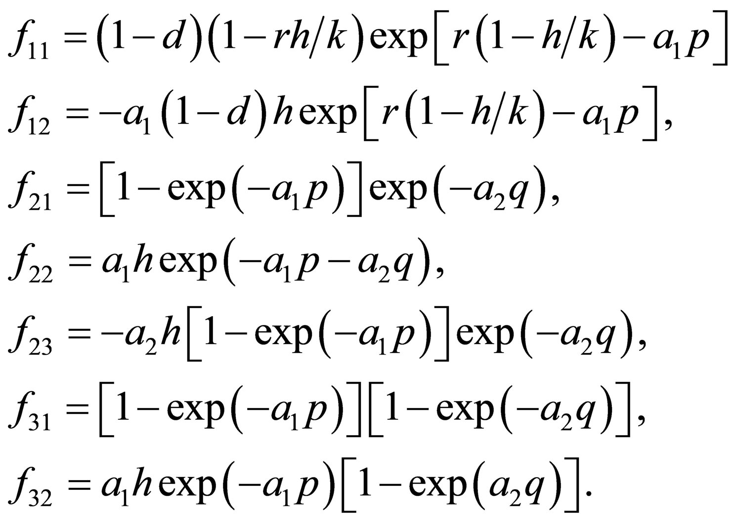
and  respectively. Now we study the linear stability of fixed points in the system (7). The Jacobian matrix at an arbitrary
  is given by
 where
where
The characteristic equation of  is
is
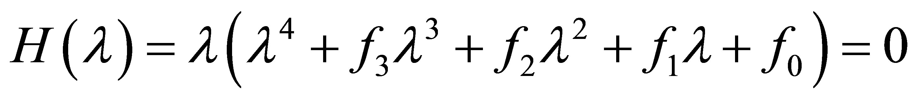 , (8)
, (8)
where
Moreover, an application of the local stability analysis of the system (7), gives the following results:
(1) Substituting the fixed point  into the Equation (8), we get
 . (9)
. (9)
The roots of the Equation (9) are 
The modulus of  is less than one. Then
  is local stability if and only if
 which yields
 (10)
(10)
(2) Substituting the fixed point  into the equation (8), we get
 , (11)
where
 .
.
Several roots of the Equation (11) are 
 . Obviously, the modulus of
  is less than one. The modulus of
  is less than one if and only if
 (12)
(12)
Under the conditions of (2) and (12), the stability of  is identified by the equation
 . (13)
It follows from the well-known Schur-cohn criterion [23] that the modulus of all roots of the Equation (13) is less than one if and only if
 . (14)
From the inequalities (12) and (14), we obtain the following conditions for the stability of :
:
Proposition 1. The equilibrium point  is locally stable if and only if the following conditions hold:
 . (15)
Proof. From the conditions (15), we can know the inequalities (2) and (12) obviously hold. Let's study the inequalities (14).
1) .
.
2) .
.
When , according to the conditions (15)we obtain
 .
.
When , according to the conditions (15), we obtain
 .
.
3) .
.
Obviously,
Therefore, if the conditions (15) are satisfied, the equilibrium point  is locally stable.
(3) Substituting the fixed point  into the Equation (8), we get
 (16)
(16)
where

Two roots of the Equation (16) are 
 . Obviously, the modulus of
  is less than one. The modulus of
  is less than one if and only if
 . (17)
Under the conditions of (4) and (17), the stability of  is identified by the equation
 . (18)
By analogy with the above, the modulus of all roots of the Equation (18) is less than one if and only if
 (19)
(19)
are satisfied. Based on the above analysis, we obtain the following sufficient conditions for the stability of .
.
Proposition 2. The equilibrium point  is locally stable if the following conditions hold:


Proof. We only need verify the inequalities (19). According to the condition , we obtain
 .
.
Substitute the signs of  and
and , we get
 ,
, . Substituting the values of
 ,
,  for
for  and rearranging the term we get
According to the condition , we obtain
 . By analogy with
 , we get
 .
.
According to the signs of , we obtain
 . Now, we prove the fourth inequality of (19).
 .
.
According to the conditions  and
and , we obtain
 . That is to say
 . At the same time,
 . The proof is complete.
(4) Substituting the fixed point  into the equation (8), we get
 , (20)
where

Under the condition of (6), the stability of  is identified by the following equation
 (21)
(21)
According to Schur-cohn criterion [23], the modulus of all roots of the Equation (21) is less than one if and only if
 (22)
(22)
are satisfied. Based on the above analysis, we obtain the following sufficient conditions for the stability of .
.
Proposition 3. Under the condition of (6), the equilibrium point  is locally stable if the following conditions hold:

where

Proof. According to the condition , we obtain
 . Substitute the signs of
 ,
,  and
and , we get
 ,
, . Substitute the values of
 ,
,  and
and , we get
 By the conditions
  and
and , we obtain
 ,
,  and
and . Then, it is easy to verify
 . And.
According to the condition , we obtain
 . That is to say
 . According to the conclusion
 , we obtain
 . Now, we prove the fifth inequality of (22).

By the condition , we obtain
The proof is complete.
3. Numerical Simulations
In this section, we use the bifurcation diagrams, the Maximum Lyapunov exponents, phase portraits and so on to explore the possibilities of dynamical behaviors for system (1).
3.1. Bifurcation Analysis
In the section, a one-dimensional bifurcation analysis is carried out to investigate the overall dynamic behavior of the system. One-dimensional bifurcation diagrams give information about the dependence of the dynamics on a certain parameter. The analysis is expected to reveal the type of attractor to which the dynamics will ultimately settle down after passing an initial transient phase and within which the trajectory will then remain forever [2]. The bifurcation parameters are considered in the following two cases:
1) Varying  in the range
 , and keeping other parameters fixed as below:
 ,
,  ,
,  ,
,  ,
, . (23)
2) Varying  in the range
  , and keeping other parameters fixed as below:
 ,
,  ,
,  ,
,  ,
, . (24)
Figure 1(a)" target="_self">Figure 1(a) shows the bifurcation diagram in the  space with the parameters given by case 1). As
  increases from
  to
to , the system is chaotic. Subsequently the chaotic attractor abruptly disappears and a period-4 attractor appears which constitute a type of attractor crisis. In the range
  , the system passes through a quasi-periodic band with frequency-lockings and tangent bifurcations. As
  further increases, a period-2 attractor appears. When
  increases from
  to
to , the system goes through a quasi-periodic band with frequency-locking and tangent bifurcation. As
  is slightly beyond
 , a stable coexistence of the system is observed. When
  increases beyond
 , the system crosses a chaotic band. When
  is slightly increased beyond
 , the hyperparasite population is extinct, while the parasitoid population enters another chaotic band with period windows. Figure 1(b)" target="_self">Figure 1(b) is the local amplifications of Figure 1(a)" target="_self">Figure 1(a) with
 .
.
The Maximum Lyapunov exponents have been proved to be the most useful dynamic diagnostic tool for chaotic systems. It is the average exponential rate of divergence or convergence of nearby orbits in phase space [24]. The Maximum Lyapunov exponents corresponding to Figure 1(a)" target="_self">Figure 1(a) are given in Figure 1(c)" target="_self">Figure 1(c), which are in agreement with the bifurcation diagram. When , the Maximum Lyapunov exponents change from positive to negative, which corresponds with the system changing from chaos to period. In the range
 , the Lyapunov exponents fluctuate around 0 with very small
Figure 1 .(a) Bifurcation diagram in  space; (b) The magnified part with
 ; (c) The Maximum Lyapunov exponents corresponding to (a). The other parameters are fixed as Equations (23).
amplitude standing for quasi-periodicity, which are the same as in the range . As
. As  increases from
  to
to , the Maximum Lyapunov exponents are negative, corresponding to a stable coexistence of the system. When
  is slightly increased beyond
 , Most of the Maximum Lyapunov exponents are positive and few are negative. So there exist period windows in the chaotic band.
As can be seen from Figure 1, the behaviors of the system are very complicated, including stable coexistence, chaotic bands with period windows, quasi-periodicity with frequency-locking. Furthermore, from an ecological point of view, it is apparent that appropriate prolonged diapause rate can moderate coexistence. The reason is that appropriate diapause rate helps the fraction hosts to escape parasitism, but high diapause goes against the parasitoid growth.
Figure 2(a)" target="_self">Figure 2(a) shows the bifurcation diagram in the  plane with the parameters given by case (Ⅱ). As the parameter
  increases from
  to
to , a stable coexistence of the system is observed. As
  further increases, a Hopf bifurcation occurs at
 . Then the system enters quasi-periodicity, including frequency-lockings and tangent bifurcations. When
 , the quasi-periodicity attractor abruptly disappears. In the range
 , there is a cascade of period-doubling bifurcations leading to chaos, which is
the same as in the range . A typical chaotic attractor is presented in Figure 2(b)" target="_self">Figure 2(b) at
 . Subsequently the chaotic attractor abruptly disappears and a period-2 attractor appears. When
  increases from 4.145 to 4.5, the system enters a chaotic band again. Figure 2(c)" target="_self">Figure 2(c) is the local amplifications of Figure 2(a)" target="_self">Figure 2(a) with
 .
.
From Figure 2, we can know that appropriate intrinsic growth rate  can stabilize the system, but the high intrinsic growth rate may destabilize the stable dynamics into more complex dynamic. The reason is that the population would increase over carrying capacity with high intrinsic growth rate and then lose its stability.
3.2. Intermittent Chaos and Supertransients
Intermittency as illustrated in Figure 3(a) is characterized by switches between apparently regular and chaotic behaviors even though all the control parameters are constant and no external noise is present [25]. The switching seems random although the dynamic model is deterministic, and the behavior is completely aperiodic and chaotic.
Figure 3(b) shows an example of supertransients, which are used to denote an unusually long convergence to an attractor. These transient dynamics are considerably longer than the timescale of significant environmental perturbations [26], because the timescale of ecological
interest is tens or hundreds of generations while supertransients can persist thousands of generations or even longer. In Figure 3(b), the hyperparasite population size suddenly stabilizes into a 4-periodic attractor after about 720 generations of complicated fluctuations.
4. Conclusion
In this paper, we have proposed and investigated the host-parasitoid-hyperparasite system with prolonged diapause for host. The existence and stability of the nonnegative fixed points are explored. Subsequently, numerical simulations are carried out to exhibit other complex dynamics including stable coexistence, quasi-periodicity, period-doubling bifurcations, and chaotic bands with periodic windows, quasiperiodic attractor and non-unique attractor, intermittent chaos and supertransients and so on. Furthermore, these simulated results are explained according to ecological perspective. From Figure 1, we can know that the system coexists with . That is to say, appropriate diapause rate is better for the stability of the system. Low diapause rate makes the host population suffer from high parasitism risk. High diapause rate goes against the parasitoids growth. These two cases destabilize the system. From Figure 2, we can know that the system is stable with
 , but the high intrinsic growth rate may destabilize the stable dynamics into more complex dynamic. The host population would increase over carrying capacity with high intrinsic growth rate and then make the whole system lose its stability.
NOTES
#Corresponding author.