Efficient Solutions of Coupled Matrix and Matrix Differential Equations ()
1. Introduction
Linear matrix and matrix differential equations show up in various fields including engineering, mathematics, physics, statistics, control, optimization, economic, linear system and linear differential system problems. For instance, the Lyapunov equations  and
and  (where A* is the conjugate transpose of A) are used to analyze of the stability of continuous-time and discrete-time systems, respectively [1]. The generalized Lyapunov equation:
 . (1)
. (1)
(where  is the transpose of B) has been used to characterize structured covariance matrices [2]. Most of the existing results, however, are connected with particular systems of such matrix and matrix differential equations.
Coupled matrix and matrix differential equations have also been widely used in stability theory of differential equations, control theory, communication systems, perturbation analysis of linear and non-linear matrix equations and other fields of pure and applied mathematics and also recently in the context of the analysis and numerical simulation of descriptor systems. For instance, the canonical system
 (2)
(2)
With the boundary conditions and  has been used to the solution of optimal control problem with the performance index [3]. In addition, many interesting problems lead to coupled Riccati matrix differential equations [4]:
 (3)
(3)
and the general class of non-homogeneous coupled matrix differential equations:
 (4)
(4)
where  are given scalar matrices,
  is a given matrix function,
  are the unknown diagonal matrix functions to be solved and
 ; and where
  denotes the derivative of matrix function
 .
. . (where
  is the set of all
  matrices over the complex number field
  and when
 , we write
  instead of
 ).
).
Examples of such situation are singular [5] and hybrid system control [6] and nonzero sum differential games [7]. Depending on the problem considered, different coupling terms may appear. However, in all the above mentioned cases the systems are difficult to solve.
Let us recall some concepts that will be used below.
Given two matrices  and
and 
 , then the Kronecker product of A and B is defined by (e.g. [8-12])
 . (5)
. (5)
While if ,
,  , and let
  and
and  be the columns of A and B, respectively, namely
 ,
, .
.
The columns of the Kronecker product  are
are  for all i, j combinations in lexicographic order namely,
 (6)
(6)
Thus, the Khatri-Rao product of A and B is defined by [13,14]:
 (7)
(7)
consists of a subset of the columns of . Notice that
  is of order
  and
and  is of order
 . This observation can be expressed in the following form [15]:
 , (8)
, (8)
where the selection matrix  is of order
  and
and
 (9)
(9)
and  is an
is an  column vector with a unity element in the k-th position and zeros elsewhere
 .
.
Additionally, if both matrices  and
and 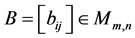 have the same size, then the Hadamard product of A and B is defined by [8-11,16]:
 . (10)
This product is much simpler than Kronecker and Khatri-Rao products and it can be connected with isomorphic diagonal matrix representations that can have a certain interest in many fields of pure and applied mathematics, for example, Tauber [16] applied the Hadamard product to solving a partial differential equation coming from an air pollution problem. The Hadamard product is clearly commutative, associative, and distributive with respect to addition. It has been known that  is a (principal) submatrix of
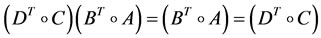
  if A and B are (square) of the same size. This can be found in Visick [12] and even in Zhang’s book [17]. Liv-Ari [13, Theorem 3.1, p. 128] gave the following new relations related to Kronecker, Khatri-Rao and Hadamard products:
 ; (11)
 . (12)
The Kronecker product and vector operator affirming their capability of solving some matrix and matrix differential equations. Such equations can be readily converted into the standard linear equation form by using the well-known identity (e.g. [17,18]):
 , (13)
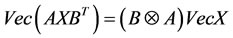
Where  denotes a vectorization by columns of a matrix. The need to compute the
 ,
,  and
and  are due its appearance in the solutions of coupled matrix differential equations. Here
 (14)
(14)
For any matrix , the spectral representation of
  and
and  assures that [9,18]:
 (15)
(15)
where  and
and  are the eigenvalues and the corresponding eigenvectors of A, and
  is the eigenvectors of matrix
 .
.
Finally, for any matrices A, B, C,  , we shall make a frequent use the following properties of the Kronecker product (e.g. [9,18-20]) which are used to establish our results.
1)
 (16)
(16)
2) ;
; ;
;
 (17)
(17)
3) ;
;
 (18)
(18)
4) ;
;
 . (19)
In this paper, we present the efficient solution of coupled matrix linear least-squares problem and extend the use of diagonal extraction (vector) operator in order to construct a computationally-efficient solution of nonhomogeneous coupled matrix linear differential equations.
2. Coupled Matrix Linear Least-Squares Problem
The multistatic antenna array processing problem can be written in matrix notation as [13]
 . (20)
where ,
,  and
and  are given (complex valued) matrices; and where the unknown matrix
  is diagonal. We also assume that n < mp, so that we suggest using a least-squares approach, viz.,
 , (21)
where  is called Frobenius norm of A. Using the identity in Equation (13) we can transform (21) into the vector LSP form:
 . (22)
which has the well-known solution:
 , (23)
provided  is invertible.
Applying the direct vector transformation in Equation (13) to  results in a highly inefficient leastsquare problem, because VecX is very sparse. Liv-Ari [13] described an alternative approach based on:
 , X is diagonal (24)
which involves the so-called Khatri-Rao product , as well as the diagonal extraction operator
 :
:
 (25)
(25)
which forms a column vector consisting of the diagonal elements of the  square matrix X, instead of the much longer column vector VecX. In addition, if Y is any matrix of order
 , then
 . (26)
As we have observed earlier, when the unknown matrix X is diagonal, solving for VecX is highly inefficient, since most of the elements of X vanish. Instead Liv-Ari [13] used the more compact vectorization identity to rewrite matrix LSP (21) in the vector form:
 . (27)
Notice that  consists of only the nontrivial (i.e., diagonal) elements of the matrix X. The explicit solution of (27) is
 . (28)
provided  is invertible.
It turns out that this expression can also be implemented using Hadamard product, resulting in a significant reduction in computational cost, as implied the following result [13]:
 , (29)
where  and
and .
.
When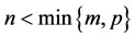 , we observe that the left-hand side expression in Equation (29) requires
  multiplications, while forming the equivalent right-hand side expression requires only
  multiplications. Thus the latter offers significant computational savings, especially when
 .
.
Now, using (26) we can rewrite (28) in the more compact form:
 . (30)
This expression which requires 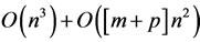 (multiply and add) operations is much more efficient than (28), which requires
  operations. It means that the computational advantage of using the Hadamard product expression is particularly evident when
 , which implies that
  . In order to be able to use (30) we must ascertain that the matrix
  is invertible. This will hold, for instance, when both A and B have full column rank.
As for the diagonal extraction operator , we observe that for any square
  matrix
 ,
,
 . (31)
If Y is diagonal, then we also have
 , Y is diagonal. (32)
Moreover, the columns of the  selection matrix
  are mutually orthonormal, viz.,
 . (33)
Using (32) and (11), we get the fundamental relation between the Hadamard product and diagonal extraction operator  which is given by
 , X is diagonal (34)
where A, B and X is  diagonal matrix.
Now we will discuss the efficient and more efficient least-squares solutions of coupled matrix linear equations:
 ,
, (35)
(35)
where A, 
 , E,
, E,  are given scalar matrices and X,
  are unknown matrices to be solved. We also assume that
 , so that the coupled matrix linear Equations (35) is over-determined, which suggests using a least squares approach. We consider the coupled matrix linear least-squares problem (CLSP):
 . (36)
The solution procedure presented here may be considered as a continuation of the method proposed to solve least-squares problem in (21).
Using the identity (13) we can transform (36) into the vector CLSP form [10]:
 (37)
(37)
which has the following solution
 (38)
(38)
One can easily show that
 (39)
(39)
where  is a unitary matrix. So
 (40)
(40)
Suppose that  and
and , we then have
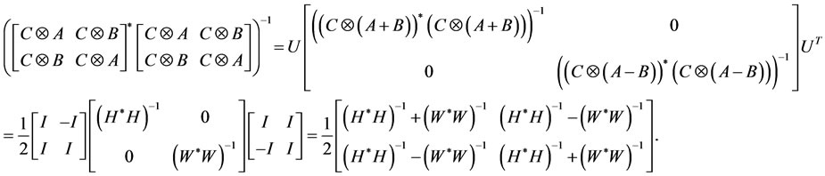 (41)
(41)
Now the least—squares solutions (38) can be rewrite into the form:
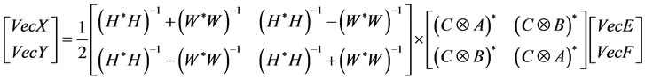 . (42)
This gives
 (43)
(43)
where  and
and .
.
In order to be able to use (38) and (43) we must ascertain that the matrix:

is invertible if and only one

and

are invertible matrices.
As we observed, when the unknown matrices X and  are diagonal, solving for VecX and VecY are highly inefficient, since most of the elements of X and Y vanish. Instead we can use the more compact vectorization identity (24) to rewrite the coupled matrix linear least-squares problem (37) in the reduced-order vector form:
 . (44)
Notice that  and
and  consists of only the nontrivial (i.e., diagonal) elements of matrices X and Y. The explicit efficient solution of (44) is
 (45)
(45)
where  and
and .
.
In order to be able to use (45), we must ascertain that the matrix

and

are invertible matrices.
It turns out that the expression (45) can also be implemented using Hadamard product by the same technique in the expression (30). Note that the least squares solutions in term of Hadamard product is more efficient than (45) and (43).
3. Non-Homogeneous Matrix Differential Equations
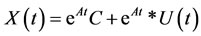
The solution procedure presented here may be considered as a continuation of the method proposed to solve the homogenous coupled matrix differential equations in [18]. We will use our knowledge of the solution of the of simplest homogeneous matrix differential equation:
 ,
, (46)
(46)
where ,
,  are given scalar matrices, and
  is the unknown matrix function to be solved. In fact the unique solution of (46) is given by:
 . (47)
Theorem 3.1 Let ,
,  are given scalar matrices,
  is a given matrix function and
  is the unknown matrix. Then the general solution of the non-homogeneous matrix differential equation:
 ,
, (48)
(48)
is given by
 . (49)
Where  is well-definedwhich involves the convolution product of two matrices
  and
and .
.
Proof: Suppose that  is the particular solution of (48). The product rule of differentiation gives
 .
.
Substituting these in (48) we obtain

Thus
 . (50)
Multiplying both sides of (50) by  gives
gives
 (51)
(51)
Integrating both sides of (51) between 0 and t gives
 (52)
(52)
Hence, by assumption, we conclude that the particular solution of equation (48) is
 . (53)
Now from (47) and (53) we get (49).
Theorem 3.2 Let ,
,  ,
,  are given scalar matrices,
  is a given matrix function and
  is unknown diagonal matrix function. Then the general solution of non-homogeneous matrix differential equation
 (54)
(54)
is given by
 . (55)
Proof: Using the identity (34) we can transform (54) into the vector form:
 (56)
(56)
Now, applying (49), then the unique solution of (56) is

If we put  in Theorem 3.2 we obtain the following result.
Corollary 3.3 Let A, B,  are given scalar matrices. Then general solution of the homogeneous matrix differential equation:
 (57)
(57)
is given by
 (58)
(58)
Now we will discuss the general class of non-homogeneous coupled matrix differential equations which defined in (4): By using the  -notation of (4), we have
 . (59)
Let
 (60)
(60)
Now (59) can be written as

and the general solution is given by:
 . (61)
Note that there is many special cases can be considered from the above general class coupled matrix differential equations; now we will discuss some important special cases in the next results.
Theorem 3.4 Let A, B, C, D, E,  are given scalar matrices such that
 ;
; 
are given matrix functions and ,
,  are the unknown diagonal matrices. Then the general solution of non-homogeneous coupled matrix differential equations:
 (62)
(62)
is given by
 (63)
(63)
Proof: Using the identity (34) we can transform (62) into the vector form:
 (64)
(64)
From (61), this system has the following solution:
 . (65)
Now we will deal with
 . (66)
Since , then we have

Then

But
 ;
;
 .
.
So
 (67)
(67)
Due to (67) we have
 ; (68)
 . (69)
Now substitute (68) and (69) in (65), we get (63).
If we put  in Theorem 3.4 we obtain the following result.
Corollary 3.5 Let A, B, C, D, E,  are given scalar matrices such that
 and
and ,
,  are the unknown diagonal matrices. Then the general solution of homogeneous coupled matrix differential equations:
 (70)
(70)
is given by
 (71)
(71)
Corollary 3.6 Let ,
,  , E,
, E,  are given scalar matrices and
 ,
,  are the unknown diagonal matrices. Then the general solution of homogeneous coupled matrix differential equations:
 (72)
(72)
is given by
 (73)
(73)
Proof: For any matrix , it is easily to show that
 ; (74)
 . (75)
Now put  in Corollary 3.5 we have

Similarly,
 .
.
While if we applying the fundamental relation between  and Kronecker product defined in (13) and using the same technique in the proof of Theorem 3.4 we obtain (for any matrix
 ) the following result.
Theorem 3.7 Let A, B, C, D, E,  are given scalar matrices such that
 ,
,  ,
,  ,
,  are given matrix functions and
 ,
,  are the unknown matrices. Then the general solution of non-homogeneous coupled matrix differential equations:
 (76)
(76)
is given by
 (77)
(77)
If we put  and
and  in Theorem 3.7 and using properties (16)-(19) we obtain the following results.
Corollary 3.8 Let B, D, E,  are given scalar matrices such that
  and
and ,
,  are the unknown matrices. Then the general solution of homogeneous coupled matrix differential equations:
 (78)
(78)
is given by
 (79)
(79)
Corollary 3.9 Let A, C, E,  are given scalar matrices such that
  and
and ,
,  are the unknown matrices .Then the general solution of homogeneous coupled matrix differential equations:
 (80)
(80)
is given by
 (81)
(81)
4. Concluding Remarks
We have studied an explicit characterization of the mappings
in terms of the selection matrix  as in (11) and (12). We have also observed that the same matrix relates the two operators
  and
and  as in (31) and (32). We used the fundamental relation between the Hadamard (Kronecker) product and diagonal extraction (vector) operator in (34) and (13) to derive our main results in Section 2 and 3 and, subsequently, to construct a computationally-efficient solution of coupled matrix least-squares problem and non-homogeneous coupled matrix differential equations. In fact, the Kronecker (Hadamard) product and operator
  (
( ) affirming their capability of solving matrix and matrix differential equations fast (more fast when the unknown matrices are diagonal). To demonstrate the usefulness of applying some properties of the Kronecker products, suppose we have to solve, for example, the following system:
 , (82)
where A,  are given scalar matrices and
  is unknown matrix to be solved. Then it is not hard by using the
  -notation to establish the following equivalence:
 , (83)
and thus also by using the  -notation product to establish the following equivalence:
 , X is diagonal. (84)
If we ignore the Kronecker (Hadamard) product structure, then we need to solve the following both matrix equations:
• (85)
(85)
Here, Y can be obtained in  arithmetic operations (flops) by using LU factorization of matrix B (Forward Substitution).
• (86)
(86)
Here X can be obtained also in  operations (flops) by using LU factorization of matrix A (Back Substitution).
Now without exploiting the Kronecker product structure, an  system defined in (82) would normally (by Gaussian elimination) require
  operations to solve. But when we use Kronecker product structure:
 , the calculations shows that
  can be obtained only in
  operations by using LU factorization of matrices A and B [20, pp. 87]. We can say that the system of the form:
  can be solved fast and the Kronecker structure also a voids the formation of
  matrices, only the smaller lower and upper triangular matrices LA, LB, UA, UB are needed. While if X is
  diagonal matrix and use the Hadamard product structure:
 , the calculations shows that
  can be obtained only in
  operations by using LU factorization of
 .
.
We can say that the system of the form:  can be solved more fast than Kronecker structure, only the very smaller lower and upper triangular matrices
  and
and  are needed. For example, consider A, B are 3 × 3 matrices and C is 9 × 1 vector. To demonstrate the usefulness of applying Kronecker product and
  -notation, we return to the system problem
 . If
. If  is non-singular and regarding with LU factorizetions of
  and
and , then a solution of system exists and can be written as:
 . (87)
First, the lower triangular system  can be solved by forward substitution as the following:

i.e.,
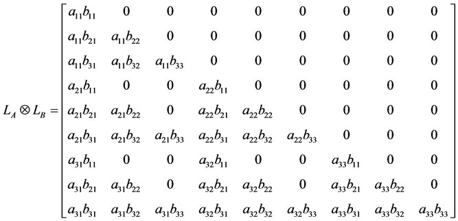
which can be solved in  operations. The first three equations are:
• . (88)
• . (89)
•
 (90)
(90)
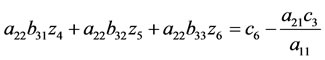
Now the next three equations are:
• . (91)
• . (92)
•
 . (93)
The first boldface expression  in (91) can be computed as
 . The second boldface expression
  in (92) can be also computed as
 .
.
While the third boldface expression  in (93) can be also computed as
 .
.
We use the previous expressions for obtaining ,
,  and
and  in the first set of equations to simplify the second set of three equations. The simplified second set of equations becomes
 . (94)
 . (95)
 . (96)
Solving the second set of equations takes  operations and the forward solve step takes
  operations, so obtaining z4, z5 and z6 takes
  time. This simplification and using the work from the previous solution step continuous so that solving each of n-sets of n-equations takes
  time, resulting in an overall solution time of
 . Exploiting the Kronecker structure reduce the usual, expected
  time to solve
  to
to .
.
One final note regarding the exploitation of the Kronecker structure of the system remains. Suppose the matrices A and B are different sizes. Then, the time required to solve the system  is
is , where
  is the size of A and
  is the size of B. In our work, the modeler has some choice for the size of the A and B matrices. Thus, a wise choice would make
  small, reducing the effect of the
  term in the
  computation time.
While when X is  diagonal matrix and applying
  -notation, we return to the system problem:
 . If
. If  is non-singular matrix and regarding with LU factorizations of
 , then a solution of system exists and can be written as:
 . (97)
First, the lower triangular system  can be solved by forward substitution as the following:
 which can be solved in
  operations as follows:
• . (98)
• . (99)
• . (100)
5. Conclusion
The solution of coupled matrix linear least-squares problems and coupled matrix differential equations is studied and some important special cases are discussed. The analysis indicates that solving for  is efficient and solving for
  is more efficient when the unknown matrices are diagonal. Although the algorithms are presented for non-homogeneous coupled matrix and matrix linear differential equations, the idea adopted can be easily extended to study coupled matrix nonlinear differential equations, e.g., the coupled matrix Riccati differential equations.
6. Acknowledgements
The author expresses his sincere thanks to referee (s) for careful reading of the manuscript and several helpful suggestions. The author also gratefully acknowledges that this research was partially supported by Deanship of Scientific Research/University of Dammam/Kingdom of Saudi Arabia/under the Grant No. 2012152.