Improved Robust Low-Rank Regularization Tensor Completion

Xiangyi Wang¹, Wei Jiang^1,2

¹School of Mathematics, Liaoning Normal University, Dalian, China.
²College of Computer Science and Artificial Intelligence, Wenzhou University, Wenzhou, China.

DOI: 10.4236/oalib.1109425                

Abstract

In recent years, there are many surrogates for tensor tubal rank. In this paper, we propose a hybrid norm consisting of the weighted nuclear norm and the weighted Frobenius norm (WTNFN) of a tensor. The WTNFN is a surrogate for tensor tubal rank, and studies the weighted tensor nuclear and Frobenius norm minimization (WTNFNM) problem. The aim is to enhance the stability of the solution and improve the shortcomings of the traditional method of minimizing approximate rank functions based on the tensor nuclear norm (TNN) in the field of low-rank tensor recovery. Based on this definition, we build a novel model for typical tensor recovery problems i.e. the weighted tensor nuclear and Frobenius tensor completion (WTNFNTC). The experimental results on synthetic data and real data show that the stability and recovery effects of the model are improved compared with related algorithms.

Keywords

Low-Rank Recovery, T-SVD, Weighted Tensor Nuclear, Weighted Tensor Frobenius Norm

1. Introduction

With the development of modern computer information technology, various data have emerged in many application fields such as mobile Internet, statistics, and psychometrics. These data are not only huge in scale, but also have the remarkable characteristics of extremely high dimensionality and complex structure. As a natural representation of multi-dimensional data, tensors are the generalization of 1-order vectors and 2-order matrices in higher-order forms [1].

In recent years, the research interest in tensors has expanded to many fields: e.g., computer vision [2], machine learning [3], pattern recognition [4], signal processing and image processing [5] [6]. For example, in a video recommendation system, user rating data can be expressed as a 3-order tensor of “user × video × time” [7]; a color image is a 3-way object with column, row and color modes. Compared with vectors and matrices, in these applications, tensors can better retain the intrinsic structure information of high-dimensional spatial data. But the tensor of interest is frequently low-rank, or approximately so [8], and hence has a much lower-dimensional structure. This motivates the low-rank tensor approximation and recovery problem. The core of the low-rank tensor recovery model is the tensor rank minimization.

In matrix processing, the rank minimization is NP-hard and is difficult to solve, the problem is generally relaxed by substitutively minimizing the nuclear norm of the estimated matrix, which is a convex relaxation of minimizing the matrix rank [9]. However, as a high-level extension of vectors and matrices, whether there is also a method similar to the matrix LMRA for low-rank tensor approximation and how to extend the low-rank definition from a matrix to a tensor is still a question worth studying. Because the notions of the tensor nuclear norm, and even tensor rank, are still ambiguous or nonuniform.

The most two popular tensor rank definitions are the CANDECOMP/PARAFAC(CP)-rank, which is related to the CANDECOMP/ PARAFAC decomposition [10], and Tucker-rank, which is corresponding to the Tucker decomposition [11] [12]. The CP rank is defined as the smallest number of rank one tensor decomposition, where the computation is generally NP-hard [13] and its convex relaxation is intractable. For the Tucker rank minimization, Liu et al. [14] first proposed the sum of nuclear norms (SNN) of unfolding matrices of a tensor to approximate the sum of Tucker rank of a tensor for tensor completion. Unfortunately, albeit the tucker rank and its convex relaxation are tractable and widely used, its direct unfolding and folding operation tend to damage intrinsic structure information of the tensor and SNN is not the convex envelope of the tucker rank according to [15].

Recently, Kilmer et al. [16] focused on a new tensor decomposition paradigm, namely tensor singular value decomposition (T-SVD), which is similar to the singular value decomposition of matrix. By using T-SVD, Kilmer et al. [16] defined the concept of tensor tubal rank, which is based on tensor-product (t-product) and its algebraic framework. T-SVD allows the matrix analysis to be extended to the tensor, while avoiding the inherent information loss in matricization or flattening of the tensor. The tensor tubal rank can well characterize the intrinsic structure of a tensor, and thus, solving low-tubal-rank related problems starts to attract more and more reasonable research interest these years.

This work focuses on the low-tubal-rank tensor recovery problem under the T-SVD framework. For the underlying tensor with low-tubal-rank assumption, it can be recovered by solving the following optimization:

$\underset{\mathcal{X}}{\min }f\left(\mathcal{X}\right)+\tau \cdot ran{k}_t\left(\mathcal{X}\right)$ (1)

where $\tau >0$ is a regularization parameter, $ran{k}_t(\cdot )$ denotes the tensor tubal rank.

It has been proved that solving (1) is NP-hard. The commonly used convex relaxation for the rank function is the tensor nuclear norm. In the recent work [17], Lu et al. first defined the tensor average rank and deduced that a tensor always has low average rank if it has low tubal rank and then proposed a novel tensor nuclear norm that is proven to be the convex envelope of the tensor average rank within the unit ball of the tensor spectral norm, which performed much better than other types of tensor nuclear norm in many tasks. This methodology is called as tensor nuclear norm minimization (TNNM). The nuclear norm of a tensor $\mathcal{X}\in {ℝ}^{n_1\times n_2\times n_3}$, denoted by ${\Vert \mathcal{X}\Vert }_{\star }$. The TNNM [17] approach has been attracting significant attention due to its rapid development in both theory and implementation. A general TNNM problem can be formulated as

$\underset{\mathcal{X}}{\min }f\left(\mathcal{X}\right)+\tau \cdot {\Vert \mathcal{X}\Vert }_{\star }$ (2)

However, even though tensor nuclear norm relaxation is becoming a popular scheme for the low-tubal-tensor recovery problem, it is also associated with shortcoming. The tensor nuclear norm suffers from the major limitation that all singular values are simultaneously minimized, which implies that large singular values are penalized more heavily than small ones. Under this circumstance, method based on nuclear norms usually fails to find a good solution. Even worse, the resulting global optimal solution may deviate significantly from the ground truth. In order to break through the limitations of the tensor nuclear norm relaxation method, there is currently work to solve the low-tubal-rank recovery problem by employing a weighted tensor nuclear norm and nonconvex relaxation strategy. The essence of relaxation is to overcome the unbalanced punishment of different singular values. Essentially, they will keep the larger singular values larger and shrink the smaller singular values. Hence, the method has already been well studied and applied in many low-tubal-rank tensor recovery problems, and in real applications, weighted tensor nuclear norm relaxation methods usually perform better than tensor nuclear norm relaxation. In addition, for low-rank representation, the Frobenius norm has been shown to perform similarly to the nuclear norm [18] [19].

This paper mainly studies the tensor completion problem. Different from the existing nonconvex tensor completion models, this paper also considers the stability and low rank of the solution of the tensor recovery model, and proposes a relatively stable low-rank nonconvex approximation of tensors. Specifically, our contributions can be summarized in the following three points.

・ First, Similar to the tensor nuclear norm definition form, we show that the square of the tensor Frobenius norm can be defined as the sum of its singular value squares. Based on the above definition, assign different weights to singular values of a tensor. We propose a surrogate of the tensor tubal rank, i.e., the WTNFN.

・ Second, to optimize the WTNFN-based minimization Problem, we extend the weighted tensor nuclear and Frobenius norm singular value thresholding (WTNFNSVT) operator which is given with careful derivations. For the tensor in the complex field, and demonstrate that it is the exact solution to the WTNFN-based minimization problem. The bounded convergence is also demonstrated with strict proof.

・ Third, we adapt the proposed weighted tensor nuclear and Frobenius norm model to different computer vision tasks. In tensor completion the model outperforms TNN methods in both PSNR index and visual perception. The proposed WTNFN-TC models also achieve better performance than traditional algorithms, especially, the low-rank learning methods designed for these tasks. The global optimal solution obtained above is relatively stable compared to existing weighted nuclear norm models.

The rest of this paper proceeds as follows: Section II briefly introduces some notations, preliminaries, and some preliminary works; Section III analyzes the optimization of the WTNFNM models, including the basic WTNFN operator in detail, and the convergences of the proposed methods are specifically analyzed with strict formulation; Section IV applies the WTNFNM model to tensor completion and compares the proposed algorithm with numerical experiments demonstrate the effectiveness of the proposed methods compared with other state-of-the-art methods; finally the conclusions and future work are given in Section V.

2. Notations and Preliminaries

2.1. Notations

We denote tensors by boldface Euler script letters, e.g., $\mathcal{A}$. Matrices are denoted by boldface capital letters, e.g., $A$, vectors are denoted by boldface lowercase letters, e.g., $a$, and scalars are denoted by lowercase letters, e.g., a. Real and complex numbers are in $ℝ$ and $ℂ$ fields respectively. For a 3-way tensor $\mathcal{A}\in {ℝ}^{n_1\times n_2\times n_3}$, we denote $\mathcal{A}\left(i,\mathrm{<mo>\; :\; </mo>,\; <mo>\; :\; </mo>}\right)$, $\mathcal{A}\left(\mathrm{<mo>\; :\; </mo>,}i,\mathrm{<mo>\; :\; </mo>}\right)$, and $\mathcal{A}\left(\mathrm{<mo>\; :\; </mo>,\; <mo>\; :\; </mo>,}i\right)$ as the i-th horizontal, lateral and frontal slice. Generally, the frontal slice $\mathcal{A}\left(\mathrm{<mo>\; :\; </mo>,\; <mo>\; :\; </mo>,}i\right)$ can also be denoted as $A^{\left(i\right)}$. We denote its $\left(i\mathrm{,}j\mathrm{,}k\right)$ -th entry as $\mathcal{A}\left(i\mathrm{,}j\mathrm{,}k\right)$ or ${\mathcal{A}}_{ijk}$. The tube is denoted $\mathcal{A}\left(i\mathrm{,}j\mathrm{,\; <mo>\; :\; </mo>}\right)$. The inner product between $A$ and $B$ in $A\in {ℝ}^{n_1\times n_2}$, is defined as $\langle A\mathrm{,}B\rangle =\text{Tr}\left(A^{\ast }B\right)$, where $\text{Tr}(\cdot )$ stands for the trace, and $A^{\text{T}}$ is the conjugate transpose of $A$, and the inner product of any two tensors $\mathcal{A}$ and $\mathcal{B}$ in ${ℂ}^{n_1\times n_2\times n_3}$, $\langle \mathcal{A}\mathrm{,}\mathcal{B}\rangle ={\displaystyle {\sum }_{i=1}^{n_3}}\langle A^{\left(i\right)}\mathrm{,}{B}^{\left(i\right)}\rangle$.

For any $\mathcal{A}\in {ℂ}^{n_1\times n_2\times n_3}$, the complex conjugate of $\mathcal{A}$ is denoted as $conj\left(\mathcal{A}\right)$ which takes the complex conjugate of each entry of $\mathcal{A}$. $\lceil b\rceil$ is the nearest integer greater than or equal to b. Now we consider applying the Discrete Fourier Transformation (DFT) on tensors. $\bar{\mathcal{A}}$ is the result of the Discrete Fourier Transformation of $\mathcal{A}$ along the third dimension, that is,

$\bar{\mathcal{A}}=fft\left(\mathcal{A}\mathrm{,}\left[\right]\mathrm{,3}\right)$ (3)

We denote $\bar{A}\in {ℂ}^{n_1{n}_3\times n_2{n}_3}$ as a block diagonal matrix with its i-th block on the diagonal as the i-th frontal slice ${\bar{A}}^{\left(i\right)}$ of $\mathcal{A}$,. i.e.,

$\bar{A}=\text{bdiag}\left(\bar{\mathcal{A}}\right)=\left[\begin{array}{cccc}{\bar{A}}^{\left(1\right)}& & & \\ & {\bar{A}}^{\left(2\right)}& & \\ & & \ddots & \\ & & & {\bar{A}}^{\left(n_3\right)}\end{array}\right]$ (4)

Next, we define the block circulant matrix $\text{bcirc}\left(\mathcal{A}\right)$ reshapes tensor $\mathcal{A}\in {ℝ}^{n_1\times n_2\times n_3}$ into a block circulant matrix with size $n_1{n}_3\times n_2{n}_3$, i.e.,

$\text{bcirc}\left(\mathcal{A}\right)=\left[\begin{array}{cccc}{A}^{\left(1\right)}& A^{\left(n_3\right)}& \cdots & A^{\left(2\right)}\\ A^{\left(2\right)}& A^{\left(1\right)}& \cdots & A^{\left(3\right)}\\ ⋮& ⋮& \ddots & ⋮\\ A^{\left(n_3\right)}& A^{\left(n_3-1\right)}& \cdots & A^{\left(1\right)}\end{array}\right]$ (5)

2.2. T-Product and T-SVD

For tensor $\mathcal{A}\in {ℝ}^{n_1\times n_2\times n_3}$, $\text{unfold}\left(\mathcal{A}\right)$ unfolds tensor $\mathcal{A}$ as follows:

$\text{unfold}\left(\mathcal{A}\right)=\left[\begin{array}{c}{A}^{\left(1\right)}\\ A^{\left(2\right)}\\ ⋮\\ A^{\left(n_3\right)}\end{array}\right]\mathrm{,}\text{fold}\left(\text{unfold}\left(\mathcal{A}\right)\right)=\mathcal{A}$ (6)

According to [17], t-product is equivalent to the familiar matrix multiplication in the Fourier domain.i.e., $\mathcal{C}=\mathcal{A}\ast \mathcal{B}$ is equivalent to $\bar{\mathcal{C}}=\bar{\mathcal{A}}\cdot \bar{\mathcal{B}}$. Then the tensor product of two third-order tensors can be defined as follows:

Definition 1 (T-product [16]) Let $\mathcal{A}\in {ℝ}^{n_1\times n_2\times n_3}$ and $\mathcal{B}\in {ℝ}^{n_1\times m\times n_3}$. Then the t-product $\mathcal{C}=\mathcal{A}\ast \mathcal{B}$ is defined to be a tensor of size $n_1\times m\times n_3$

$\mathcal{C}=\mathcal{A}\ast \mathcal{B}=\text{fold}\left(\text{bcirc}\left(\mathcal{A}\right)\cdot \text{unfold}\left(\mathcal{B}\right)\right)$ (7)

Definition 2 (Conjugate Transpose [16]) The conjugate transpose of a tensor of $\mathcal{A}\in {ℂ}^{n_1\times n_2\times n_3}$ size $n_1\times n_2\times n_3$ is a $n_2\times n_1\times n_3$ tensor ${\mathcal{A}}^{\text{T}}$ obtained by conjugate transposing each of the frontal slice and then reversing the order of transposed frontal slices 2 through $n_3$. If tensor is $\mathcal{A}\in {ℝ}^{n_1\times n_2\times n_3}$, Conjugate transpose is also recorded as ${\mathcal{A}}^{\text{T}}$.

Definition 3 (Identity Tensor [16]) The identity tensor $\mathcal{I}\in {ℝ}^{n\times n\times n_3}$ is the tensor whose first frontal slice is an $n\times n$ identity matrix, and whose other frontal slices are all zeros.

Definition 4 (Orthogonal Tensor [16]) A tensor $\mathcal{Q}\in {ℝ}^{n\times n\times n_3}$ is orthogonal if it satisfies

${\mathcal{Q}}^{\text{T}}\ast \mathcal{Q}=\mathcal{Q}\ast {\mathcal{Q}}^{\text{T}}=\mathcal{I}$ (8)

Definition 5 (F-diagonal Tensor [16]) A tensor is called F-diagonal if each of its frontal slices is a diagonal matrix.

As stated above, tensor-SVD can be defined.

Theorem 1 (T-SVD [17]) Let $\mathcal{A}\in {ℝ}^{n_1\times n_2\times n_3}$. Then it can be factorized as

$\mathcal{A}=\mathcal{U}\ast \mathcal{S}\ast {\mathcal{V}}^{\text{T}}$ (9)

where $\mathcal{U}\in {ℝ}^{n_1\times n_1\times n_3}$, $\mathcal{V}\in {ℝ}^{n_2\times n_2\times n_3}$ are orthogona tensors, and $\mathcal{S}\in {ℝ}^{n_1\times n_2\times n_3}$ is an F-diagonal tensor.

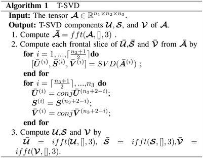
It is worth noting that T-SVD can be efficiently computed based on the matrix SVD in the Fourier domain. The details of T-SVD are described in Algorithm 1.

Definition 6 (Tensor Tubal Rank [20] [21]) For $\mathcal{A}\in {ℝ}^{n_1\times n_2\times n_3}$, the tensor tubal rank, denoted as $ran{k}_t\left(\mathcal{A}\right)$, is defined as the number of nonzero singular tubes of $\mathcal{S}$, where $\mathcal{S}$ is from the T-SVD of $\mathcal{A}=\mathcal{U}\ast \mathcal{S}\ast {\mathcal{V}}^{\text{T}}$. The tensor tubal rank is equivalent to the number of nonzero singular values of $\mathcal{A}$. That is

$ran{k}_t\left(\mathcal{A}\right)=\mathrm{<mo>\; \#\; </mo>}\left\{i\mathrm{,}\mathcal{S}\left(i\mathrm{,}i\mathrm{,\; <mo>\; :\; </mo>}\right)\ne 0\right\}=\mathrm{<mo>\; \#\; </mo>}\left\{i\mathrm{,}\mathcal{S}\left(i\mathrm{,}i\mathrm{,1}\right)\ne 0\right\}\mathrm{.}$ (10)

where $\mathcal{S}\left(i\mathrm{,}i\mathrm{,1}\right)=\frac{1}{n_3}{\displaystyle {\sum }_{j=1}^{n_3}}\bar{\mathcal{S}}\left(i\mathrm{,}i\mathrm{,}j\right)$, it uses the property induced by inverse DFT. Denote $\sigma \left(\mathcal{A}\right)\in {ℝ}^{n\times n_3}$ with ${\sigma }_{ij}\left(\mathcal{A}\right)=\bar{\mathcal{S}}\left(i\mathrm{,}i\mathrm{,}j\right)$, therefore, the Tensor unclear norm and Frobenius norm tensor are defined as follows.

Definition 7 (Tensor Nuclear Norm (TNN) [22]) For tensor $\mathcal{A}\in {ℝ}^{n_1\times n_2\times n_3}$, based on the result about the tensor nuclear norm derived from the T-product. we have the tensor nuclear norm (TNN) is defined to be

${\Vert \mathcal{A}\Vert }_{\star }=\frac{1}{n_3}{\displaystyle \underset{i=1}{\overset{m}{\sum }}{\displaystyle \underset{j=1}{\overset{n_3}{\sum }}{\sigma }_{ij}\left(\mathcal{A}\right)}}$ (11)

Theorem 2 (Tensor Frobenius Norm (TFN)) Given a tensor $\mathcal{A}\in {ℝ}^{n_1\times n_2\times n_3}$, if $\mathcal{A}=\mathcal{U}\ast \mathcal{S}\ast {\mathcal{V}}^{\text{T}}$ the following hold:

${\Vert \mathcal{A}\Vert }_F=\frac{1}{\sqrt{n_3}}{\displaystyle \underset{i=1}{\overset{m}{\sum }}{\displaystyle \underset{j=1}{\overset{n_3}{\sum }}\sqrt{{\sigma }_{ij}^2\left(\mathcal{A}\right)}}}$ (12)

3. Proposed Algorithm Scheme

Based on the definition of tensor nuclear norm and tensor Frobenius norm in Definition 8 and Theorem 2, we present a new nonconvex regularizer which is defined as the sum of the weighted tensor nuclear norm and the square of the weighted tensor Frobenius norm (WTNFN) of $\mathcal{X}\in {ℝ}^{n_1\times n_2\times n_3}$

$\begin{array}{c}{\Vert \mathcal{X}\Vert }_{\text{WTNFN}}={\Vert \mathcal{X}\Vert }_{W\mathrm{,}\star }+\gamma {\Vert \mathcal{X}\Vert }_{W\mathrm{,}F}^2\\ =\frac{1}{n_3}{\displaystyle \underset{i=1}{\overset{m}{\sum }}{\displaystyle \underset{j=1}{\overset{n_3}{\sum }}{w}_{ij}{\sigma }_{ij}\left(\mathcal{X}\right)}}+\frac{\gamma }{n_3}{\displaystyle \underset{i=1}{\overset{m}{\sum }}{\displaystyle \underset{j=1}{\overset{n_3}{\sum }}{w}_{ij}{\sigma }_{ij}^2\left(\mathcal{X}\right)}}\end{array}$ (13)

where $W={\left(w_{ij}\right)}_{n\times n_3}$ is the weight matrix, $n=\min \left(n_1\mathrm{,}{n}_2\right)$, $\gamma$ is a positive parameter.

3.1. Problem Formulation

Consider the general weighted tensor nuclear and Frobenius norm framework for tensor tubal rank minimization problems

$\underset{\mathcal{X}}{\min }f\left(\mathcal{X}\right)+\tau \cdot {\Vert \mathcal{X}\Vert }_{\text{WTNFN}}$ (14)

where $\mathcal{X}\in {ℝ}^{n_1\times n_2\times n_3}$, $\tau >0$ is a positive parameter. And the loss function $f\left(\mathcal{X}\right)$ satisfy the following assumptions:

・ $f:{ℝ}^{n_1\times n_2\times n_3}\to {ℝ}^{+}$ is continuously differentiable with Lipschitz continuous gradient, i.e., for any $\mathcal{X}\mathrm{,}\mathcal{Y}\in {ℝ}^{n_1\times n_2\times n_3}$

${\Vert \nabla f\left(\mathcal{X}\right)-\nabla f\left(\mathcal{Y}\right)\Vert }_F\le L\left(f\right)\Vert \mathcal{X}-\mathcal{Y}\Vert$ (15)

where $L\left(f\right)>0$ is the Lipschitz constant.

・ f is coercive, i.e., $f\left(\mathcal{X}\right)\to \infty$ when $\mathcal{X}\to \infty$.

To enhance low rank, we need to design a scheme to keep the weights of large singular values sufficiently small and the weights of small singular values sufficiently large, which will lead to a nearly unbiased low rank approximation. Intuitively, one can set each weight, which the entries of matrix $w_{ij}\in {ℝ}^{+}$ to be inversely proportional to the corresponding singular value ${\sigma }_{ij}\left(\mathcal{X}\right)$, which will penalize large singular values less and overcome the unfair penalization of different singular values.

3.2. Methodology

We solve problem (14) by generating an iterative sequence ${\mathcal{X}}^{\left(k\right)}$, where ${\mathcal{X}}^{\left(k+1\right)}$ is the minimizer of a weighted tensor nuclear and Frobenius norm regularized problem that comes from the linearized approximation of the objective function $f\left(\mathcal{X}\right)$ at ${\mathcal{X}}^{\left(k\right)}$. To realize this, for the loss function $f\left(\mathcal{X}\right)$, we approximate it as a quadratic function

$f\left(\mathcal{X}\right)=f\left({\mathcal{X}}^{\left(k\right)}\right)+\langle \nabla f\left({\mathcal{X}}^{\left(k\right)}\right)\mathrm{,}\mathcal{X}-{\mathcal{X}}^{\left(k\right)}\rangle +\frac{{\mu }^{\left(k\right)}}{2}{\Vert \mathcal{X}-{\mathcal{X}}^{\left(k\right)}\Vert }_F^2$ (16)

Since optimizing $f\left(\mathcal{X}\right)$ directly is hard, we minimize its approximation (16) instead. Hence, we solve the following relaxed problem to update ${\mathcal{X}}^{\left(k+1\right)}$

$\begin{array}{c}{\mathcal{X}}^{\left(k+1\right)}=\underset{\mathcal{X}}{\arg \min }f\left({\mathcal{X}}^{\left(k\right)}\right)+\langle \nabla f\left({\mathcal{X}}^{\left(k\right)}\right)\mathrm{,}\mathcal{X}-{\mathcal{X}}^{\left(k\right)}\rangle \\ +\frac{{\mu }^{\left(k\right)}}{2}{\Vert \mathcal{X}-{\mathcal{X}}^{\left(k\right)}\Vert }_F^2+\tau \cdot {\Vert {\mathcal{X}}^{\left(k\right)}\Vert }_{\text{WTNFN}}\end{array}$ (17)

By ignoring constant terms and combining others, (17) can be expressed equivalently as

${\mathcal{X}}^{\left(k+1\right)}=\frac{{\mu }^{\left(k\right)}}{2\tau }{\Vert \mathcal{X}-\left({\mathcal{X}}^{\left(k\right)}-\frac{1}{{\mu }^{\left(k\right)}}\nabla f\left({\mathcal{X}}^{\left(k\right)}\right)\right)\Vert }_F^2+\tau \cdot {\Vert {\mathcal{X}}^{\left(k\right)}\Vert }_{\text{WTNFN}}$ (18)

Thus, consider ${\mathcal{Y}}^{\left(k\right)}={\mathcal{X}}^{\left(k\right)}-\frac{1}{{\mu }^{\left(k\right)}}\nabla f\left({\mathcal{X}}^{\left(k\right)}\right)$ the above formula is equivalent

to the following, which is a nonconvex proximal operator problem. Next, we will prove (18) has a closed-form solution by exploiting the special structure of it.

3.3. WTNFNSVT Operator

The weighted tensor nuclear and Frobenius norm singular value thresholding (WTNFNSVT) operator is defined as follows to compute the proximal minimizer of the tensor weighted nuclear and Frobenius norm minimization.

Theorem 3 (WTNFNSVT Operator) Let $\mathcal{Y}=\mathcal{U}\ast \mathcal{S}\ast {\mathcal{V}}^{\text{T}}$ be the T-SVD of $\mathcal{Y}\in {ℝ}^{n_1\times n_2\times n_3}$. For any $\tau >0$, $\gamma >0$, the solution of the problem

$\underset{\mathcal{X}}{\min }{\Vert \mathcal{X}-\mathcal{Y}\Vert }_F^2+\tau \cdot {\Vert \mathcal{X}\Vert }_{\text{WTNFN}}$ (19)

is given by ${\mathcal{D}}_{W\mathrm{,}\gamma }$, which is defined the WTNFNSVT operator as

${\mathcal{D}}_{W\mathrm{,}\gamma }=\mathcal{U}\ast {\mathcal{S}}_{W\mathrm{,}\gamma }\ast {\mathcal{V}}^{\text{T}}$ (20)

where ${\mathcal{S}}_{W\mathrm{,}\gamma }=ifft\left({\left({\left(1+\gamma \tau \mathcal{W}\right)}^{-1}\left(\bar{\mathcal{S}}-\frac{\tau }{2}\mathcal{W}\right)\right)}_{+}\mathrm{,}\left[\right]\mathrm{,3}\right)$, $\mathcal{W}\in {ℝ}^{n_1\times n_2\times n_3}$ is F-diagonal whose diagonal entries of the j-th frontal slice are equal to the j-th column of weight matrix $W$. The entries of weight matrix $W$ satisfies $0\le w_{1j}\le w_{2j}\le \cdots \le w_{nj}$, $n=\min \left[n_1,n_2\right]$, $j=1,2,\cdots ,n_3$.

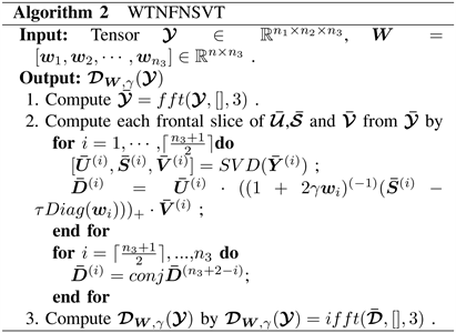
Theorem 2 shows that the WTNFNSVT operator ${\mathcal{D}}_{W\mathrm{,}\gamma }$ gives a close-from of the proximal minimizer of the WTNFN minimization with monotone nonnegative weights, which is a natural extension of the weighted matrix SVT. The feasibility of this extension is guaranteed by the T-SVD framework. Using Algorithm 1, we show how to compute ${\mathcal{D}}_{W\mathrm{,}\gamma }$ efficiently in Algorithm 2.

Obviously, when $\gamma =0$ the weighted tensor nuclear norm minimization (WTNNM) was a special case of this problem at that time. And secondly, when all weights were set the same, tensor nuclear norm minimization (TNNM) was a special case of this problem. Therefore, the solution of this model covers the solutions of traditional TNNM and WTNNM.

3.4. The Setting of Weighting Matrix

In previous sections, we proposed to utilize the WTNFNM model and its solving method. By introducing the weight vector, the WTNFNM model improves the flexibility of the original TNNM model. However, the weight vector itself also brings more parameters in the model. Appropriate setting of the weights plays a crucial role in the success of the proposed WTNFNM model.

Inspired by the weighted unclear norm proposed by Gu et al. [23], a similar weighting method can be used in the weighted tensor unclear norm and Frobenius norm, that is

$w_{ij}^{k+1}=\frac{C}{{\sigma }_{ij}\left({\mathcal{X}}^{\left(k\right)}\right)+\epsilon }$ (21)

where ${\sigma }_{ij}\left({\mathcal{X}}^{\left(k\right)}\right)$ is the singular value of the tensor $\mathcal{X}$ in the k-th iteration, $w_{ij}^{k+1}$ is the corresponding weight of ${\sigma }_{ij}\left({\mathcal{X}}^{\left(k\right)}\right)$. Because (21) is monotonically decreasing with the singular values, the non-descending order of weights with respect to singular values will be kept throughout the reweighting process. According to the Remark 1 in [23], we can get Corollary 1 as follow:

Corollary 1. Let $\mathcal{Y}=\mathcal{U}\ast \mathcal{S}\ast {\mathcal{V}}^{\text{T}}$ be the T-SVD of tensor $\mathcal{Y}\in {ℝ}^{n_1\times n_2\times n_3}$, ${\sigma }_{ij}\left(\mathcal{Y}\right)\mathrm{<mo>\; :\; </mo>}=\bar{\mathcal{S}}\left(i\mathrm{,}i\mathrm{,}j\right)$ denotes singular value of the tensor $\mathcal{Y}$. If the regularization parameter C is positive and the positive value $\epsilon$ is small enough. By using

the reweighting formula $w_{ij}^{k+1}=\frac{C}{{\sigma }_{ij}\left({\mathcal{X}}^{\left(k\right)}\right)+\epsilon }$, and initial estimate ${\mathcal{X}}^{\left(0\right)}=\mathcal{Y}$. The reweighted problem

$\underset{\mathcal{X}}{\min }\Vert \mathcal{X}-\mathcal{Y}\Vert +\tau \cdot \left({\Vert \mathcal{X}\Vert }_{w,\star }+\gamma {\Vert \mathcal{X}\Vert }_{w,F}^2\right)$ (22)

has a closed-form solution

$\hat{\mathcal{X}}=\mathcal{U}\ast {\mathcal{S}}_w\ast {\mathcal{V}}^{\text{T}}$ (23)

where ${\mathcal{S}}_w$ is a F-diagonal tensor, ${\sigma }_{ij}\left(\mathcal{X}\right)\mathrm{<mo>\; :\; </mo>}={\bar{\mathcal{S}}}_w\left(i\mathrm{,}i\mathrm{,}j\right)$. Consider $c_1=\tau \left({\sigma }_j\left({\bar{Y}}^{\left(i\right)}\right)-\epsilon -\gamma C\right)$ and $c_2={\tau }^2{\left({\sigma }_j\left({\bar{Y}}^{\left(i\right)}\right)-\epsilon -\gamma C\right)}^2-4\left(2C-\tau \epsilon {\sigma }_j\left({\bar{Y}}^{\left(i\right)}\right)\right)$. We get

${\sigma }_{ij}\left(\hat{\mathcal{X}}\right)=\{\begin{array}{ll}0\hfill & \text{if}{c}_2>0\hfill \\ \frac{c_1+\sqrt{c_2}}{2}\hfill & \text{if}{c}_2>0\hfill \end{array}$ (24)

The proof of Corollary 1 can be found in supplementary material. Corollary 1 shows that although a reweighting strategy (21) is used, we do not need to iteratively perform the thresholding and weight calculation operations. In each iteration of both the WTNFNM models to solve the typical tensor recovery problems, and the tensor completion algorithms, such a reweighting strategy is performed on the WTNFNSVT subproblem (step 2 in Algorithms 2) to adjust weights based on current ${\mathcal{X}}^{\left(k\right)}$. In implementation, we initialize ${\mathcal{X}}^{\left(0\right)}$ as the observation tensor $\mathcal{Y}$. The above weight setting strategy greatly facilitates the WTNFNM calculations. Note that there remain two parameters C and $\gamma$ in the WTNFNM implementation. In all of our experiments, we set it by experience for certain tasks. Please see the following sections for details.

3.5. Convergence Analysis

In this section, we give the convergence analysis for (18). Suppose that the sequence ${\mathcal{X}}^{\left(k\right)}$ is generated by Algorithm 2. For the simplicity of notation, we denote ${\sigma }_{ij}^k$ as the singular value of $\mathcal{X}$ in the k-th iteration, and $w_{ij}^k$ is the corresponding weight of ${\sigma }_{ij}^k$.

Theorem 4. In problem (14), assume that $f\left(\mathcal{X}\right)$ satisfy the assumptions and $\nabla f$ is Lipschitz continuous. Consider $F\left(\mathcal{X}\right)=f\left(\mathcal{X}\right)+\tau \cdot {\Vert \mathcal{X}\Vert }_{\text{WTNFN}}$, and the parameter ${\mu }^{\left(k\right)}\ge \frac{L\left(f\right)}{1-\tau \alpha }$ for any $k\ge 0$, $0<\alpha <1$. Then the sequence $\left\{{\mathcal{X}}^{\left(k\right)}\right\}$ and $\left\{F\left({\mathcal{X}}^{\left(k\right)}\right)\right\}$ generated by WTNFNM satisfies the following properties:

1) $F\left({\mathcal{X}}^{\left(k\right)}\right)$ is monotonically decreasing. Indeed,

$F\left({\mathcal{X}}^{\left(k\right)}\right)-F\left({\mathcal{X}}^{\left(k+1\right)}\right)\le \frac{{\mu }^{\left(k\right)}-L\left(f\right)}{1-2\tau }{\Vert {\mathcal{X}}^{\left(k+1\right)}-{\mathcal{X}}^{\left(k\right)}\Vert }_F^2$ (25)

2) The sequence $\left\{{\mathcal{X}}^{\left(k\right)}\right\}$ is always bounded. Moreover, $\underset{k\to +\infty }{\lim }\left({\mathcal{X}}^{\left(k+1\right)}-{\mathcal{X}}^{\left(k\right)}\right)=0$.

3) Any accumulation point $\hat{\mathcal{X}}$ of the sequence $\left\{{\mathcal{X}}^{\left(k\right)}\right\}$ is a critical point of $F\left(\mathcal{X}\right)$.

Proof. (1) First, with the definition of ${\mathcal{X}}^{\left(k+1\right)}$, i.e.,

${\mathcal{X}}^{\left(k+1\right)}=\arg \underset{\mathcal{X}}{\min }\frac{{\mu }^{\left(k\right)}}{2\tau }{\Vert \mathcal{X}-\left({\mathcal{X}}^{\left(k\right)}-\frac{1}{\mu }\nabla f\left({\mathcal{X}}^{\left(k\right)}\right)\right)\Vert }_F^2+{\Vert \mathcal{X}\Vert }_{\text{WTNFN}}$ (26)

We have

$\begin{array}{c}{X}^{\left(k+1\right)}=\arg \underset{\mathcal{X}}{\min }\frac{1}{n_3}{\displaystyle \underset{i=1}{\overset{m}{\sum }}{\displaystyle \underset{j=1}{\overset{n_3}{\sum }}\left(w_{ij}^{\left(k\right)}{\sigma }_{ij}+w_{ij}^{\left(k\right)}{\sigma }_{ij}^2\right)}}+\frac{{\mu }^{\left(k\right)}}{2\tau }{\Vert \mathcal{X}-\left({\mathcal{X}}^{\left(k\right)}-\frac{1}{\mu }\nabla f\left({\mathcal{X}}^{\left(k\right)}\right)\right)\Vert }_F^2\\ =\arg \underset{\mathcal{X}}{\min }\frac{1}{n_3}{\displaystyle \underset{i=1}{\overset{m}{\sum }}{\displaystyle \underset{j=1}{\overset{n_3}{\sum }}\left(w_{ij}^{\left(k\right)}{\sigma }_{ij}+w_{ij}^{\left(k\right)}{\sigma }_{ij}^2\right)}}+\langle \nabla f\left({\mathcal{X}}^{\left(k\right)}\right)\mathrm{,}\mathcal{X}-{\mathcal{X}}^{\left(k\right)}\rangle \\ +\frac{{\mu }^{\left(k\right)}}{2\tau }{\Vert \mathcal{X}-{\mathcal{X}}^{\left(k\right)}\Vert }_F^2\end{array}$

Then

$\begin{array}{l}\frac{1}{n_3}{\displaystyle \underset{i=1}{\overset{m}{\sum }}{\displaystyle \underset{j=1}{\overset{n_3}{\sum }}\left(w_{ij}^{\left(k\right)}{\sigma }_{ij}^{\left(k+1\right)}+w_{ij}^{\left(k\right)}{\left({\sigma }_{ij}^{\left(k+1\right)}\right)}^2\right)}}\\ +\langle \nabla f\left({\mathcal{X}}^{\left(k\right)}\right)\mathrm{,}{\mathcal{X}}^{\left(k+1\right)}-{\mathcal{X}}^{\left(k\right)}\rangle +\frac{{\mu }^{\left(k\right)}}{2\tau }{\Vert {\mathcal{X}}^{\left(k+1\right)}-{\mathcal{X}}^{\left(k\right)}\Vert }_F^2\\ \le \frac{1}{n_3}{\displaystyle \underset{i=1}{\overset{m}{\sum }}{\displaystyle \underset{j=1}{\overset{n_3}{\sum }}\left(w_{ij}^{\left(k\right)}{\sigma }_{ij}^{\left(k\right)}+w_{ij}^{\left(k\right)}{\left({\sigma }_{ij}^{\left(k\right)}\right)}^2\right)}}\\ +\langle \nabla f\left({\mathcal{X}}^{\left(k\right)}\right)\mathrm{,}{\mathcal{X}}^{\left(k\right)}-{\mathcal{X}}^{\left(k\right)}\rangle +\frac{{\mu }^{\left(k\right)}}{2\tau }{\Vert {\mathcal{X}}^{\left(k\right)}-{\mathcal{X}}^{\left(k\right)}\Vert }_F^2\end{array}$

which can be rewritten as

$\begin{array}{l}\langle \nabla f\left({\mathcal{X}}^{\left(k\right)}\right)\mathrm{,}{\mathcal{X}}^{\left(k+1\right)}-{\mathcal{X}}^{\left(k\right)}\rangle \\ \le \frac{1}{n_3}{\displaystyle \underset{i=1}{\overset{m}{\sum }}{\displaystyle \underset{j=1}{\overset{n_3}{\sum }}\left(w_{ij}^{\left(k\right)}\left({\sigma }_{ij}^{\left(k\right)}-{\sigma }_{ij}^{\left(k+1\right)}\right)+\left({\left({\sigma }_{ij}^{\left(k\right)}\right)}^2-{\left({\sigma }_{ij}^{\left(k+1\right)}\right)}^2\right)\right)}}-\frac{{\mu }^{\left(k\right)}}{2\tau }{\Vert {\mathcal{X}}^{\left(k+1\right)}-{\mathcal{X}}^{\left(k\right)}\Vert }_F^2\end{array}$ (27)

Second, note that f is Lipschitz gradient continuous. According to [ [24] Lemma 2.11], we have

$f\left({\mathcal{X}}^{\left(k+1\right)}\right)-f\left({\mathcal{X}}^{\left(k\right)}\right)\le \langle \nabla f\left({\mathcal{X}}^{\left(k\right)}\right)\mathrm{,}{\mathcal{X}}^{\left(k+1\right)}-{\mathcal{X}}^{\left(k\right)}\rangle +\frac{L\left(f\right)}{2}{\Vert {\mathcal{X}}^{\left(k+1\right)}-{\mathcal{X}}^{\left(k\right)}\Vert }_F^2$ (28)

Finally, we combine (27) and (28), it obtains that

$\begin{array}{l}F\left({\mathcal{X}}^{\left(k+1\right)}\right)-F\left({\mathcal{X}}^{\left(k\right)}\right)\\ =\frac{1}{n_3}{\displaystyle \underset{i=1}{\overset{m}{\sum }}{\displaystyle \underset{j=1}{\overset{n_3}{\sum }}\left(w_{ij}^{\left(k+1\right)}\left({\sigma }_{ij}^{\left(k+1\right)}-{\left({\sigma }_{ij}^{\left(k+1\right)}\right)}^2\right)+w_{ij}^{\left(k\right)}\left({\sigma }_{ij}^{\left(k\right)}-{\left({\sigma }_{ij}^{\left(k\right)}\right)}^2\right)\right)}}\\ +f\left({\mathcal{X}}^{\left(k+1\right)}\right)-f\left({\mathcal{X}}^{\left(k\right)}\right)\\ \le \frac{1}{n_3}{\displaystyle \underset{i=1}{\overset{m}{\sum }}{\displaystyle \underset{j=1}{\overset{n_3}{\sum }}\left(w_{ij}^{\left(k\right)}\left({\sigma }_{ij}^{\left(k\right)}-{\sigma }_{ij}^{\left(k+1\right)}\right)+{\left({\sigma }_{ij}^{\left(k\right)}\right)}^2-{\left({\sigma }_{ij}^{\left(k+1\right)}\right)}^2\right)}}\\ +\langle \nabla f\left({\mathcal{X}}^{\left(k\right)}\right)\mathrm{,}{\mathcal{X}}^{\left(k+1\right)}-{\mathcal{X}}^{\left(k\right)}\rangle +\frac{L\left(f\right)}{2\tau }{\Vert {\mathcal{X}}^{\left(k+1\right)}-{\mathcal{X}}^{\left(k\right)}\Vert }_F^2\end{array}$

which leads

$F\left({\mathcal{X}}^{\left(k+1\right)}\right)+\frac{{\mu }^{\left(k\right)}-L\left(f\right)}{2\tau }{\Vert {\mathcal{X}}^{\left(k+1\right)}-{\mathcal{X}}^{\left(k\right)}\Vert }_F^2\le F\left({\mathcal{X}}^{\left(k\right)}\right)$ (29)

Since for any integer k, if ${\mu }^{\left(k\right)}\ge \frac{L\left(f\right)}{1-\alpha \tau }$ we have $\frac{{\mu }^{\left(k\right)}-L\left(f\right)}{2\tau }\ge \frac{\alpha }{2}{\mu }^{\left(k\right)}$ always held. Then the monotone search criterion (25) is always satisfied, which makes the $F\left({\mathcal{X}}^{\left(k\right)}\right)$ is monotonically decreasing.

2) It’s easy to obtain that $F\left({\mathcal{X}}^{\left(k\right)}\right)$ is bounded. Then, we know that $\left\{{\mathcal{X}}^{\left(k\right)}\right\}$ is bounded as well from the assumption. Besides, summing up the inequality (27) for all $k\ge 0$, it leads that

$\begin{array}{c}F\left({\mathcal{X}}^{\left(0\right)}\right)\ge {\displaystyle \underset{k=0}{\overset{+\infty }{\sum }}}\frac{{\mu }^{\left(k\right)}-L\left(f\right)}{2\tau }{\Vert {\mathcal{X}}^{\left(k+1\right)}-{\mathcal{X}}^{\left(k\right)}\Vert }_F^2\\ \ge \frac{2-2\alpha \tau }{\alpha L\left(f\right)}{\displaystyle \underset{k=0}{\overset{+\infty }{\sum }}}{\Vert {\mathcal{X}}^{\left(k+1\right)}-{\mathcal{X}}^{\left(k\right)}\Vert }_F^2\end{array}$

Hence, we get

${\displaystyle \underset{k=0}{\overset{+\infty }{\sum }}}{\Vert {\mathcal{X}}^{\left(k+1\right)}-{\mathcal{X}}^{\left(k\right)}\Vert }_F^2\le \frac{{\mu }^{\left(k\right)}-L\left(f\right)}{2\tau }<+\infty$ (30)

From (30), it yields that

$\underset{k\to +\infty }{\lim }\left({\mathcal{X}}^{\left(k+1\right)}-{\mathcal{X}}^{\left(k\right)}\right)=0$ (31)

3) Because of the boundedness of the sequence $\left\{{\mathcal{X}}^{\left(k\right)}\right\}$, there exists a subsequence $\left\{{\mathcal{X}}^{\left(k_t\right)}\right\}$ such that it converges to an accumulation point $\hat{\mathcal{X}}$, i.e., ${\lim }_{t\to +\infty }{\mathcal{X}}^{\left(k_t\right)}=\hat{\mathcal{X}}$. Based on that convergence result (31), we have ${\lim }_{t\to +\infty }{\mathcal{X}}^{\left(k_t\right)}=\hat{\mathcal{X}}$, which implies that ${\lim }_{t\to +\infty }{\sigma }_{ij}\left({\mathcal{X}}^{\left(k_t\right)}\right)={\sigma }_{ij}\left(\hat{\mathcal{X}}\right)$ for all i and j. Note that the subsequence $\left\{{\mathcal{X}}^{\left(k_t\right)}\right\}$ is bounded obviously, according to the [ [25] Proposition 2.1.5], there exists ${\hat{w}}_{ij}\in w_{ij}\left({\sigma }_{ij}\left(\hat{\mathcal{X}}\right)+{\sigma }_{ij}^2\left(\hat{\mathcal{X}}\right)\right)$ such that ${\lim }_{t\to +\infty }{w}_{ij}^{\left(k_t\right)}={\hat{w}}_{ij}$ for all i and j. Denote

$T\left(\mathcal{X}\mathrm{,}W\right)=\frac{1}{n_3}{\displaystyle \underset{i=1}{\overset{m}{\sum }}{\displaystyle \underset{j=1}{\overset{n_3}{\sum }}{w}_{ij}\left({\sigma }_{ij}\left(\mathcal{X}\right)+{\sigma }_{ij}^2\left(\mathcal{X}\right)\right)}}$ (32)

Since ${\mathcal{X}}^{\left(k_t\right)}$ is optimal to problem (30), there exists ${\mathcal{Z}}^{\left(k_t\right)}\in T\left({\mathcal{X}}^{\left(k_t\right)}\mathrm{,}{W}^{\left(k_t\right)}\right)$ such that

${\mathcal{Z}}^{\left(k_t\right)}\in T\left({\mathcal{X}}^{\left(k_t\right)}\mathrm{,}{W}^{\left(k_t\right)}\right)$ (33)

such that

${\mathcal{Z}}^{\left(k_t+1\right)}+\nabla f\left({\mathcal{X}}^{\left(k_t\right)}\right)+{\mu }^{\left(k_t\right)}\left({\mathcal{X}}^{\left(k_t+1\right)}-{\mathcal{X}}^{\left(k_t\right)}\right)=\mathcal{O}$ (34)

Let $t\to +\infty$ in the above equation, then we obtain that there exists $\hat{\mathcal{Z}}\in \partial T\left(\hat{\mathcal{X}}\mathrm{,}\hat{W}\right)$

$\mathcal{O}=\hat{\mathcal{Z}}+\nabla f\left(\hat{\mathcal{X}}\right)\in \partial F\left(\hat{\mathcal{X}}\right)$ (35)

Thus $\hat{\mathcal{X}}$ is a critical point of problem (14). This completes the proof.

4. Experiments

In this section, we conducted a series of experiments on both synthetic and real-world data to demonstrate the superiority of the proposed model. we empirically demonstrated that the WTNFN regularization algorithm leads to more stable solutions than WTNN (with $\gamma =0$ ). Moreover, it could achieve better performance when compared to the previous algorithm.

We solved the low rank tubal tensor completion problem by the following program using the Discrete Fourier Transform based tensor nuclear norm based on the proposed weighted tensor nuclear and Frobenius norm

$\underset{\mathcal{X}}{\min }\tau {\Vert \mathcal{X}\Vert }_{\text{WTNFN}}+\frac{1}{2}{\Vert {\mathcal{P}}_{\Omega }\left(\mathcal{X}\right)-{\mathcal{P}}_{\Omega }\left(\mathcal{M}\right)\Vert }_F^2\mathrm{,}$ (36)

where $\mathcal{X}\mathrm{,}\mathcal{M}\mathrm{,}\Omega$ were respectively the observed data and the underlying recover result, a binary support indicator tensor. Zeros in $\Omega$ indicate the missing entries in the observed tensor, and ${\mathcal{P}}_{\Omega }\mathrm{<mo>\; :\; </mo>}{ℝ}^{n_1\times n_1\times n_3}\to {ℝ}^{n_1\times n_1\times n_3}$ was a linear operator that keeps the entries in unchanged and sets those outside zeros. It was easy to know that the gradient of the squared loss function was a Lipschitz continuous function with a Lipschitz constant $L\left(f\right)=1$. The quality of the restored image was evaluated in terms of the peak-signal-to-noise ratio (PSNR) defined by

$\text{PSNR}=10{\log }_{10}\left(\frac{{\Vert \mathcal{M}\Vert }_{\infty }^2}{\frac{1}{n_1{n}_2{n}_3}{\Vert \hat{\mathcal{X}}-\mathcal{M}\Vert }_F^2}\right)$ (37)

4.1. Stability of the WTNFN Regularization Model

In this section, we show that WTNFN model leads to more stable solutions and provides improved experimental results than WTNN for color images. In our experiments, the testing images shown in Figure 1 were the “Im1” and “Im5” with size 300 × 300 × 3. For each image, pixels were sampled randomly with sampling rates of 30%, 50%, and 70%. These two images were used to illustrate the effectiveness of the Frobenius norm in the WTNFN.

We first applied the WTNFN with different $\gamma$ values to “Im1” and “Im5”. A suitable value of should $\gamma$ result to a stabilized solution and meanwhile result to a solution of high PSNR value. We denote WTNN the WTNN regularization model with $\gamma =0$, WTNFN1 with $\gamma$ is about 10⁻⁶, WTNFN2 with a lager $\gamma$ about 10⁻⁵. Figure 1 shows the PSNR values of sampling rates of 30%, 50%, and 70%, respectively, for recovering images “Im1” and “Im5” 10 times. Comparing the WTNFN with different values of $\gamma$, we can find that the PSNR values of WTNFN1 and WTNFN2 are more stable than that of WTNN, which indicates that the Frobenius norm in the WTNFN penalty can induce stable solutions. In addition, we found that WTNFN11 and WTNFN2 behave very similarly for the values of PSNR for the same image at the same sample rate. So we should choose moderate value of $\gamma$ to balance the stability and the quality of the restored image. The results in Figure 1 show that setting $\gamma ={10}^{-6}$ to make sure that always achieves good results.

4.2. Synthetic Experiments

We conducted an experiment to demonstrate the practical applicability of the WTNFN heuristic for recovering low-rank tensors. We generated a tensor by $\mathcal{X}=\mathcal{M}\ast \mathcal{N}$, where the entries of $\mathcal{M}\in {ℝ}^{n\times r\times n}$ and $\mathcal{N}\in {ℝ}^{r\times n\times n}$ were independently sampled from standard Gaussian distribution. The tubal rank of tensor $\mathcal{X}$ was defined as r. We solve (36) and obtain the solution $\hat{\mathcal{X}}$. Then we reported to the tubal rank $r_t$ of $\hat{\mathcal{X}}$ and Relative Error was defined as

$\text{RelativeError}\mathrm{<mo>\; :\; </mo>}=\frac{{\Vert \hat{\mathcal{X}}-\mathcal{X}\Vert }_F}{{\Vert \mathcal{X}\Vert }_F}$ (38)

We simply considered tensors of size $n\times n\times n$, with $n=\left[\mathrm{50,100,200}\right]$. To

Figure 1. Performance of the WTNFN on images “Im1” and “Im5” for different randomly sampled sets. (a) Results for sampling rate 30% “Im1”. (b) Results for sampling rate 30% “Im5”. (c) Results for sampling rate 50% “Im1”. (d) Results for sampling rate 50% “Im5”. (e) Results for sampling rate 70% “Im1”. (f) Results for sampling rate 70% “Im5”.

create the known entries, we sampled $m=p{n}^3$ items uniformly from $\mathcal{X}$, where p was the sampling rate. A reference quantity that is defined as $d_r=r\left(2n-r\right)n$ in the literature [26]. We set the parameter $\tau =0.01$, $\gamma ={10}^{-6}$ for model (36) in experiment. Table 1 respectively gives the recovery results for the linear transform DFT. It can be seen that the WTNFN program (36) gives the correct rank estimation of $\mathcal{X}$ in all cases and the relative errors are small. Therefore, these results do a good job of validating the correct recovery guarantees of our algorithm.

Next, we studied the recovery phenomenon with different tubal ranks of $\mathcal{X}$ and different sampling rates of p. We generated a 50 × 50 × 50 tensor $\mathcal{X}$ similarly to the previous experiment. The range of variations for tubal ranks r and sampling rates p were $r=\left[\mathrm{1,}\cdots \mathrm{,20}\right]$ and $p=\left[\mathrm{0.01,}\cdots \mathrm{,0.99}\right]$. The tubal rank was gradually increased in steps of 1. The sampling rate was gradually increased in steps of 0.01. We conducted an experiment for each $\left(p\mathrm{,}r\right)$ pair. The algorithms stopped when the Relative Error was less than 10⁻⁵. Figure 2 reports the percentage of success for each pair of WTNFN and TNN for the linear transform DFT, in which the yellow region reflects the full successful recovery, and the blue region reflects the full failed recovery. The bigger the yellow area, the stronger ability to recover. It can be seen that the WTNFN method has a much larger yellow area than the TNN method. The recovery phenomena can be explained by the fact that WTNFN has a stronger ability to recovery than TNN. In a word, the WTNFN minimization model is more robust and efficient than the classic TNN minimization model.

4.3. Real World Experiments

Due to coding and transmission difficulties, photos may be partially damaged or obscured by text or branding. Matrix completion methods, of course, can be used to recover the missing information in these images. We considered the

Table 1. Exact tensor completion on random data.

Figure 2. Comparison of the recovery capacity varying tubal rank r and sampling rate p of the WTNFN (a) and TNN (b). The x-axis represents the sampling rate p, ranging from 0.01 to 0.99, the y-axis represents the tubal rank r, ranging from 1 to 20.

WFNFN to color image recovery with partially missing pixels, as color images with three channels (Red, Green, Blue) can be modeled as third-order low-tubal rank tensors. The Peak Signal-to-Noise Ratio (PSNR) is a widely used measure for assessing image quality. To compare the performance of different approaches, we utilize the PSNR value of the recovered image. Larger values of PSNR indicate better image restoration performance.

We considered four methods for image recovery and compare their performance: 1) TNN-DFT [26]: tensor nuclear norm based discrete Fourier transform tensor completion model; 2) TNNR [27]: tensor truncated nuclear norm regularization; 3) L_p [22]: tensor completion by nonconvex L_p function regularization; 4) TCTF [28]: tensor completion by tensor factorization.

a) Random Mask: We first conducted experiments to deal with a relatively easy tensor completion problem. We randomly selected 5 images with a size of 300 × 300 × 3 from the LJU dataset, and randomly sampled 50% of pixels for each image.

Five recovered image examples with sampling rate of 50% by different methods are shown in “Fig.”. In the magnified views of the comparable sections in color boxes, it reveals that our recovered images have a clearer shape, fuller color, and brightness than the other four state-of-the-art tensor completion methods. Furthermore, we display the PSNR values achieved by various approaches on five images in Figure 3 when the sampling rate is 50%. It can demonstrate that the WTNFN-based algorithms can achieve much higher PSNR values compared with the other four state-of-the-art tensor completion methods quantitatively for the majority of the images.

b) Text Mask: Text removal is difficult because the pixels covered by the text are not spread evenly throughout the image, and the text may obscure essential textural information. We start by looking at the text's location and treating the

Figure 3. Five images of natural scenes.

Table 2. PSNR values of the various methods on text mask for image recovery.

Figure 4. Comparison of the PSNR values obtained by TNNDTF, TNNR, L_P, TCTF and WTNFN on the tested images in Figure 5

items that correspond to it as missing values. As a result, the text removal problem can be thought of as a tensor completion problem in general. In this experiment, we apply our method to estimate the images from text mask.

As previously noted, we compared our results to the TNN-DFT, TNNR, L_p, and TCTF methods. PSNR measurements are used to assess performance. The recovered images from the five tensor completion algorithms are shown in Figure 6. On all five image sequences, We rounded the experimental results to two decimal places. Table 2 provides the PSNR values of the compared approaches. We

Figure 5. Performance comparison for image recovery on some sample images. (a) original image; (b) observed image; (c) recovered images by TNN-DFT, (d) recovered images by TNNR, (e) recovered images by L_p, (f) recovered images by TCTF, (g) recovered images by WTNFN.

can see that the WTNFN has absolute superiority, as evidenced by its far higher PSNR values.

5. Conclusions

In this work, we have presented a novel method called the weighted nuclear and Frobenius norm regularization for low-tubal rank tensor recovery. We proposed the solving approach for the weighted nuclear and Frobenius norm proximal (WTNFNSVT) operator. The WTNFN model was subsequently extended to tensor completion tasks, and efficient algorithms were developed to solve these using the derived WTNFNSVT operator. Influenced by the weighted nuclear for automatic weight setting. We also developed a rational scheme for automatic weight setting, which yields closed from solutions of the WTNFN operator. This approach can shorten the calculation time.

On both synthetic and actual visual datasets, we ran many experiments. In comparison to state-of-the-art tensor completion approaches based on the tenor nuclear norm or tensor factorization, the experimental findings indicate the

Figure 6. Comparison of tensor completion algorithms for text removal problem. (a) original image; (b) observed image; (c) recovered images by TNN-DFT (d) recovered images by TNNR, (e) recovered images by L_p, (f) recovered images by TCTF, (g) recovered images by WTNFN.

advantages of the WTNFN-based algorithms.

Acknowledgements

This work is supported by Innovative talents support plan of colleges and universities in Liaoning Province (2021).

Appendix A. Proof of Theorem 2

Lemma 1. Given a third-order tensor $\mathcal{A}\in {ℝ}^{n_1\times n_2\times n_3}$ if $\mathcal{U}\in {ℝ}^{n_1\times n_2\times n_3}$ is orthogonal, i.e., $\mathcal{U}\ast {\mathcal{U}}^{\text{T}}={\mathcal{U}}^{\text{T}}\ast \mathcal{U}=\mathcal{I}$, that is

${\Vert \mathcal{U}\ast \mathcal{A}\Vert }_F={\Vert \mathcal{A}\ast \mathcal{U}\Vert }_F={\Vert \mathcal{X}\Vert }_F$ (39)

The theorem 2 can be proved by lemma 1.

Proof By lemma 1 and $\mathcal{A}=\mathcal{U}\ast \mathcal{S}\ast {\mathcal{V}}^{\text{T}}$ can get

${\Vert \mathcal{A}\Vert }_F={\Vert \mathcal{S}\Vert }_F=\frac{1}{\sqrt{n_3}}{\displaystyle \underset{i=1}{\overset{n}{\sum }}}{\displaystyle \underset{j=1}{\overset{n_3}{\sum }}}\sqrt{{\sigma }_{ij}^2\left(\mathcal{A}\right)}$ (40)

End of proof.

Appendix B. Proof of Theorem 3

Proof of Theorem 3 requires the following Lemma 2.

Lemma 2 (Proximal Operator for WNFN) For a matrix $X\in {ℂ}^{m\times n}\left(m>n\right)$, denote by $Y=U{\Sigma }^{\text{T}}V$ the singular value decomposition of matrix $Y$, and $0\le w_1\le w_2\le \cdots \le w_n$, the following minimization problem

$\underset{X}{\min }{\Vert X-Y\Vert }_F^2+\tau \cdot \left({\Vert X\Vert }_{w\mathrm{,}\star }+\gamma {\Vert X\Vert }_{w\mathrm{,}F}^2\right)$ (41)

The solution is $pro{x}_{{\Vert \cdot \Vert }_{w\mathrm{,}\star }+{\Vert \cdot \Vert }_{w\mathrm{,}F}^2}$,

$pro{x}_{{\Vert \cdot \Vert }_{w\mathrm{,}\star }+{\Vert \cdot \Vert }_{w\mathrm{,}F}^2}=U{S}_w\left(\Sigma \right)V^{\text{T}}$ (42)

where $S_w\left(\Sigma \right)=\max \left\{{\left(1+\gamma \tau w_i\right)}^{-1}\left({\Sigma }_{ii}-\frac{2}{\tau }{w}_i\right)\mathrm{,0}\right\}$

B1. Proof of Lemma 1

Proof In order to prove Lemma 2, we first show the following theorem for the proximal operator of weighted nuclear and Frobenius norm for real-valued matrices. Then, we extend the result to prove Lemma 2 for complex-valued matrices.

For any $X\mathrm{,}Y\in {ℝ}^{m\times n}\left(m>n\right)$, denote by $\bar{U}D{\bar{V}}^{\text{T}}$ and $U\Sigma V$ the singular value decomposition of matrix $X$ and $Y$, where $\Sigma =\left(\begin{array}{c}diag\left({\sigma }_1\mathrm{,}{\sigma }_2\mathrm{,}\cdots ,{\sigma }_n\right)\\ 0\end{array}\right)\in {ℝ}^{m\times n}$, and $D=\left(\begin{array}{c}diag\left(d_1\mathrm{,}{d}_2\mathrm{,}\cdots ,d_n\right)\\ 0\end{array}\right)$ are the diagonal singular value matrices. Based on the property of Frobenius norm, the following derivations hold:

$\begin{array}{l}{\Vert X-Y\Vert }_F^2+\tau \cdot \left({\Vert X\Vert }_{w\mathrm{,}\ast }+\gamma {\Vert X\Vert }_{w\mathrm{,}F}^2\right)\\ =\text{Tr}\left(Y^{\text{T}}Y\right)-2\text{Tr}\left(Y^{\text{T}}X\right)+\text{Tr}\left(X^{\text{T}}X\right)+\tau \cdot \left({\displaystyle \underset{i}{\overset{n}{\sum }}{w}_i{d}_i}+\gamma {\displaystyle \underset{i}{\overset{n}{\sum }}{w}_i{d}_i^2}\right)\\ ={\displaystyle \underset{i}{\overset{n}{\sum }}{\sigma }_i^2}-2\text{Tr}\left(Y^{\text{T}}X\right)+{\displaystyle \underset{i}{\overset{n}{\sum }}{d}_i^2}+\tau \cdot \left({\displaystyle \underset{i}{\overset{n}{\sum }}{w}_i{d}_i}+\gamma {\displaystyle \underset{i}{\overset{n}{\sum }}{w}_i{d}_i^2}\right)\end{array}$

Based on the von Neumann trace inequality, we know that $\text{Tr}\left(X^{\text{T}}Y\right)$ achieves its upper bound ${\displaystyle {\sum }_i^n}{\sigma }_i{d}_i$ if $U=\bar{U}$, $V=\bar{V}$. Then we have

$\underset{X}{\min }{\Vert X-Y\Vert }_F^2+\tau \cdot \left({\Vert X\Vert }_{w\mathrm{,}\ast }+\gamma {\Vert X\Vert }_{w\mathrm{,}F}^2\right)$

$\begin{array}{l}\iff \underset{D}{\min }{\displaystyle \underset{i}{\overset{n}{\sum }}{\sigma }_i^2}-2{\displaystyle \underset{i}{\overset{n}{\sum }}{\sigma }_i{d}_i}+{\displaystyle \underset{i}{\overset{n}{\sum }}{d}_i^2}+\tau \cdot \left({\displaystyle \underset{i}{\overset{n}{\sum }}{w}_i{d}_i}+\gamma {\displaystyle \underset{i}{\overset{n}{\sum }}{w}_i{d}_i^2}\right)\\ \text{s}\text{.t}.d_1\ge d_2\ge \cdots \ge d_n\ge 0\end{array}$

$\begin{array}{l}\iff \underset{D}{\min }{\displaystyle \underset{i}{\overset{n}{\sum }}{\left({\sigma }_i-d_i\right)}^2}+\tau \cdot \left(w_i{d}_i+\gamma w_i{d}_i^2\right)\\ \text{s}\text{.t}.d_1\ge d_2\ge \cdots \ge d_n\ge 0\end{array}$

From the above derivation, we can see that the optimal solution of the WNFNP problem is $X^{\star }=UD{V}^{\text{T}}$, where $D$ is the optimum of the constrained quadratic optimization problem.

The following proof holds the Lemma 2 on the complex number field.

Let $Y=Y_1+i{Y}_2\in {ℂ}^{n\times m}$ be an arbitrary complex-valued matrix and its SVD be $Y=\left(U+iP\right)\Sigma {\left(V+iQ\right)}^{\text{T}}$, where $Y_1\in {ℝ}^{n\times m}$, $Y_2\in {ℝ}^{n\times m}$, $U\in {ℝ}^{n\times n}$, $P\in {ℝ}^{n\times m}$, $\Sigma \in {ℝ}^{n_0\times n_0}$, $V\in {ℝ}^{m\times m}$, $Q\in {ℝ}^{m\times m}$, and $n_0=\left\{n\mathrm{,}m\right\}$. Then, it is easy to verify that the SVD of the matrix

$A=\left[\begin{array}{rr}\hfill Y_1& \hfill Y_2\\ \hfill -Y_2& \hfill Y_1\end{array}\right]\in {ℝ}^{2m\times 2m}$ (43)

can be expressed as

$A=\left[\begin{array}{cc}U& P\\ -P& U\end{array}\right]\left[\begin{array}{cc}\Sigma & \\ & \Sigma \end{array}\right]{\left[\begin{array}{cc}V& -Q\\ Q& V\end{array}\right]}^{\text{T}}$ (44)

Let $X=L_1+i{L}_2\in {ℂ}^{n\times m}$, $B=\left[\begin{array}{rr}\hfill L_1& \hfill L_2\\ \hfill -L_2& \hfill L_1\end{array}\right]\in {ℝ}^{2n\times 2m}$, $\tilde{w}={\left[w^{\text{T}},w^{\text{T}}\right]}^{\text{T}}\in {ℝ}_{+}^{2n_0}$, and the functions

$h_1\left(X\right)={\Vert X-Y\Vert }_F^2+\tau \cdot \left(w{\Vert X\Vert }_{\star }+\gamma w{\Vert X\Vert }_F^2\right)$ (45)

$h_2\left(B\right)=\frac{1}{2}{\Vert A-B\Vert }_F^2+\tau \cdot \left(\frac{\tilde{w}}{2}{\Vert A\Vert }_{\star }+\gamma \frac{\tilde{w}}{2}{\Vert A\Vert }_F^2\right)$ (46)

From the decomposition formula of the above matrix, $h_1\left(X\right)=h_2\left(B\right)$, According to Lemma 1, one minimizer to the following minimization problem

$\underset{B}{\min }\frac{1}{2}{\Vert A-B\Vert }_F^2+\tau \cdot \left(\frac{\tilde{w}}{2}{\Vert A\Vert }_{\star }+\gamma \frac{\tilde{w}}{2}{\Vert A\Vert }_F^2\right)$ (47)

The optimal solution is $B^{\star }=U{S}_{\tilde{w}\mathrm{,}\gamma }{V}^{\text{T}}$. Since $h_1\left(X\right)=h_2\left(B\right)$, the function $h_2\left(B^{\star }\right)$ the same minimum value as $h_2\left(X^{\star }\right)$ with $X^{\star }=U{S}_{w\mathrm{,}\gamma }{V}^{\text{T}}$.

End of proof.

B2. Proof of Theorem 3

Proof Theorem 3 describes one minimizer to the following minimization problem

$\underset{\mathcal{X}}{\min }{\Vert \mathcal{X}-\mathcal{Y}\Vert }_F^2+\tau \cdot {\Vert \mathcal{X}\Vert }_{\text{WTNFN}}\iff \underset{{\bar{X}}^{\left(i\right)}}{\min }\frac{1}{n_3}{\displaystyle \underset{i=1}{\overset{n_3}{\sum }}}\left({\Vert {\bar{X}}^{\left(i\right)}-{\bar{Y}}^{\left(i\right)}\Vert }_F^2\right)+\tau \cdot {\Vert {\bar{X}}^{\left(i\right)}\Vert }_{\text{WTNFN}}$ (48)

From Lemma 2, the optimal solution of the above formula can be expressed as

${\bar{X}}^{\left(i\right)}{}^{\star }={\bar{U}}^{\left(i\right)}{\bar{S}}_{w\mathrm{,}\gamma }^{\left(i\right)}\left({\bar{S}}^{\left(i\right)}\right){\bar{V}}^{\left(i\right)}{}^{\text{T}}$ (49)

where ${\bar{S}}_{w\mathrm{,}\gamma }^{\left(i\right)}\left({\bar{S}}^{\left(i\right)}\right)=\max \left\{{\left(1+\gamma w_{i\mathrm{,}j}\right)}^{-1}\left({\bar{S}}^{\left(i\right)}-w_{i\mathrm{,}j}\right)\mathrm{,0}\right\}$, denotes by ${\bar{Y}}^{\left(i\right)}={\bar{U}}^{\left(i\right)}{\bar{S}}^{\left(i\right)}{\bar{V}}^{\left(i\right)}{}^{\text{T}}$ the singular value decomposition of matrix ${\bar{Y}}^{\left(i\right)}$. So denotes $\bar{U}$, ${\bar{S}}_{w\mathrm{,}\gamma }$, $\bar{V}$ as three tensors. Their frontal slices are ${\bar{U}}^{\left(i\right)}$, ${\bar{S}}_{w\mathrm{,}\gamma }^{\left(i\right)}$, ${\bar{V}}^{\left(i\right)}$. Performing the inverse fast Fourier transform to get $\mathcal{U}=ifft\left(\bar{U}\mathrm{,}\left[\right]\mathrm{,3}\right)$, ${\mathcal{S}}_{w\mathrm{,}\gamma }=ifft\left({\bar{S}}_{w\mathrm{,}\gamma }\mathrm{,}\left[\right]\mathrm{,3}\right)$, $\mathcal{V}=ifft\left(\bar{V}\mathrm{,}\left[\right]\mathrm{,3}\right)$, the optimal solution as follow

$\mathcal{X}=\mathcal{U}{\mathcal{S}}_{w\mathrm{,}\gamma }{\mathcal{V}}^{\text{T}}$ (50)

End of proof.

B3. Proof of Corollary 1

Proof From Lemma 1, we can see that the weighted near-end operator problem:

$\underset{\mathcal{X}}{\min }{\Vert \mathcal{X}-\mathcal{Y}\Vert }_F^2+\tau \cdot {\Vert \mathcal{X}\Vert }_{\text{WTNFN}}=\underset{{\bar{X}}^{\left(i\right)}}{\min }\frac{1}{n_3}{\displaystyle \underset{i=1}{\overset{n_3}{\sum }}}\left({\Vert {\bar{X}}^{\left(i\right)}-{\bar{Y}}^{\left(i\right)}\Vert }_F^2\right)+\tau \cdot {\Vert {\bar{X}}^{\left(i\right)}\Vert }_{\text{WTNFN}}$ (51)

The closed form solution is

${\bar{X}}^{\left(i\right)}{}^{\star }={\bar{U}}^{\left(i\right)}{\bar{S}}_{w\mathrm{,}\gamma }^{\left(i\right)}\left({\bar{S}}^{\left(i\right)}\right){\bar{V}}^{\left(i\right)}{}^{\text{T}}$ (52)

where

${\bar{S}}_{w\mathrm{,}\gamma }^{\left(i\right)}=\left(\begin{array}{c}\text{diag}\left({\sigma }_1\left({\bar{X}}^{\left(i\right)}{}^{\star }\right),\cdots ,{\sigma }_{\min \left\{n_1,n_2\right\}}\left({\bar{X}}^{\left(i\right)}{}^{\star }\right)\right)\\ 0\end{array}\right)$ (53)

According to the updated rules of the algorithm, in each iteration, the weight $\left\{w_{i\mathrm{,}j}^{\left(k\right)}\right\}$ are in a non-descending order, and the singular values ${\sigma }_j\left({\bar{X}}^{\left(i\right)}\right)$ can be updated independently in a non-increasing order as

$\begin{array}{l}{\sigma }_j\left({\bar{X}}_k^{\left(i\right)}\right)=\max \left\{{\left(1+\gamma w_{i\mathrm{,}j}^{\left(k-1\right)}\right)}^{-1}\left({\sigma }_j\left({\bar{Y}}^{\left(i\right)}\right)-\frac{2}{\tau }{w}_{i\mathrm{,}j}^{\left(k-1\right)}\right)\mathrm{,0}\right\}\\ =\max \left\{{\left(1+\gamma C{\left({\sigma }_j\left({\bar{X}}_{k-1}^{\left(i\right)}\right)+\epsilon \right)}^{-1}\right)}^{-1}\mathrm{,}\left({\sigma }_j\left({\bar{Y}}^{\left(i\right)}\right)--\frac{2}{\tau }C{\left({\sigma }_j\left({\bar{X}}_{k-1}^{\left(i\right)}\right)+\epsilon \right)}^{-1}\right)\mathrm{,0}\right\}\end{array}$ (54)

Based on the prior condition that the weights are initialized as $w_{i\mathrm{,}j}^{\left(0\right)}=\frac{C}{{\sigma }_j\left({\bar{Y}}^{\left(i\right)}\right)+\epsilon }$, then we have

$\begin{array}{l}{\sigma }_j\left({\bar{X}}_1^{\left(i\right)}\right)=\max \left\{{\left(1+\gamma w_{i\mathrm{,}j}^{\left(0\right)}\right)}^{-1}\left({\sigma }_j\left({\bar{Y}}^{\left(i\right)}\right)-\frac{2}{\tau }{w}_{i\mathrm{,}j}^{\left(0\right)}\right)\mathrm{,0}\right\}\\ =\max \left\{{\left(1+\gamma C{\left({\sigma }_j\left({\bar{Y}}^{\left(i\right)}\right)+\epsilon \right)}^{-1}\right)}^{-1}\mathrm{,}\left({\sigma }_j\left({\bar{Y}}^{\left(i\right)}\right)--\frac{2}{\tau }C{\left({\sigma }_j\left({\bar{Y}}^{\left(i\right)}\right)+\epsilon \right)}^{-1}\right)\mathrm{,0}\right\}\\ \le {\sigma }_j\left({\bar{Y}}^{\left(i\right)}\right)\end{array}$ (55)

Since $\gamma >0,C>0$. Then in the next iteration, we have

$\begin{array}{l}{\sigma }_j\left({\bar{X}}_2^{\left(i\right)}\right)=\max \left\{{\left(1+\gamma w_{i\mathrm{,}j}^{\left(1\right)}\right)}^{-1}\left({\sigma }_j\left({\bar{Y}}^{\left(i\right)}\right)-\frac{2}{\tau }{w}_{i\mathrm{,}j}^{\left(1\right)}\right)\mathrm{,0}\right\}\\ =\max \left\{{\left(1+\gamma C{\left({\sigma }_j\left({\bar{X}}_2^{\left(i\right)}\right)+\epsilon \right)}^{-1}\right)}^{-1}\mathrm{,}\left({\sigma }_j\left({\bar{Y}}^{\left(i\right)}\right)-\frac{2}{\tau }C{\left({\sigma }_j\left({\bar{X}}_2^{\left(i\right)}\right)+\epsilon \right)}^{-1}\right)\mathrm{,0}\right\}\\ \le \max \left\{{\left(1+\gamma C{\left({\sigma }_j\left({\bar{Y}}^{\left(i\right)}\right)+\epsilon \right)}^{-1}\right)}^{-1}\mathrm{,}\left({\sigma }_j\left({\bar{Y}}^{\left(i\right)}\right)--\frac{2}{\tau }C{\left({\sigma }_j\left({\bar{Y}}^{\left(i\right)}\right)+\epsilon \right)}^{-1}\right)\mathrm{,0}\right\}\\ ={\sigma }_j\left({\bar{X}}_1^{\left(i\right)}\right)\end{array}$ (56)

Then, the weights in the first and second iteration satisfy:

$w_{i\mathrm{,}j}^{\left(2\right)}=C{\left({\sigma }_j\left({\bar{X}}_2^{\left(i\right)}\right)+\epsilon \right)}^{-1}\ge C{\left({\sigma }_j\left({\bar{X}}_1^{\left(i\right)}\right)+\epsilon \right)}^{-1}=w_{i\mathrm{,}j}^{\left(1\right)}$ (57)

Hence, in the I iteration, suppose that, holds for all the singular values, then the inequality

$\begin{array}{l}{\sigma }_j\left({\bar{X}}_{I+1}^{\left(i\right)}\right)\\ =\max \left\{{\left(1+\gamma C{\left({\sigma }_j\left({\bar{X}}_I^{\left(i\right)}\right)+\epsilon \right)}^{-1}\right)}^{-1}\mathrm{,}\left({\sigma }_j\left({\bar{Y}}^{\left(i\right)}\right)-\frac{2}{\tau }C{\left({\sigma }_j\left({\bar{X}}_I^{\left(i\right)}\right)+\epsilon \right)}^{-1}\right)\mathrm{,0}\right\}\\ \le \max \left\{{\left(1+\gamma C{\left({\sigma }_j\left({\bar{X}}_{I-1}^{\left(i\right)}\right)+\epsilon \right)}^{-1}\right)}^{-1}\mathrm{,}\left({\sigma }_j\left({\bar{Y}}^{\left(i\right)}\right)-\frac{2}{\tau }C{\left({\sigma }_j\left({\bar{X}}_{I-1}^{\left(i\right)}\right)+\epsilon \right)}^{-1}\right)\mathrm{,0}\right\}\\ ={\sigma }_j\left({\bar{X}}_I^{\left(i\right)}\right)\end{array}$ (58)

In summary, $\forall j=1,2,\cdots ,\min \left\{n_1,n_2\right\}$, $i=1,2,3,\cdots ,n_3$, ${\sigma }_j\left({\bar{X}}_k^{\left(i\right)}\right)\le {\sigma }_j\left({\bar{X}}_{k-1}^{\left(i\right)}\right)$ and $w_{i\mathrm{,}j}^{\left(k\right)}\ge w_{i\mathrm{,}j}^{\left(k-1\right)}$. Because the singular value $\left\{{\sigma }_j\left({\bar{X}}_k^{\left(i\right)}\right)\right\}$ is bounded below by 0, then the sequence is convergent. And sequence $\left\{{\sigma }_j\left({\bar{X}}_k^{\left(i\right)}\right)\right\}$ converges to a non-negative number ${\sigma }_j\left({\bar{X}}_k^{\left(i\right)\star }\right)$.

$\begin{array}{l}{\sigma }_j\left({\bar{X}}^{\left(i\right)\star }\right)=\underset{k\to \infty }{\lim }{\sigma }_j\left({\bar{X}}_k^{\left(i\right)}\right)\\ =\max \left\{{\left(1+\gamma \underset{k\to \infty }{\lim }{w}_{i\mathrm{,}j}^{\left(k\right)}\right)}^{-1}\left({\sigma }_j\left({\bar{Y}}^{\left(i\right)}\right)-\frac{2}{\tau }\underset{k\to \infty }{\lim }{w}_{i\mathrm{,}j}^{\left(k\right)}\right)\mathrm{,0}\right\}\\ ={\left(1+\gamma C{\left({\sigma }_j\left({\bar{X}}^{\left(i\right)\star }\right)+\epsilon \right)}^{-1}\right)}^{-1}\left({\sigma }_j\left({\bar{Y}}^{\left(i\right)}\right)-\frac{2}{\tau }C{\left({\sigma }_j\left({\bar{X}}^{\left(i\right)\star }\right)+\epsilon \right)}^{-1}\right)\end{array}$ (59)

Then we have

${\sigma }_j\left({\bar{X}}^{\left(i\right)\star }\right)=\{\begin{array}{l}0\text{if}{c}_2>0\\ \frac{c_1+\sqrt{c_2}}{2}\text{if}{c}_2>0\end{array}$ (60)

where $c_2={\tau }^2{\left({\sigma }_j\left({\bar{Y}}^{\left(i\right)}\right)-\epsilon -\gamma C\right)}^2-4\left(2C-\tau \epsilon {\sigma }_j\left({\bar{Y}}^{\left(i\right)}\right)\right)$ and $c_1=\tau \left({\sigma }_j\left({\bar{Y}}^{\left(i\right)}\right)-\epsilon -\gamma C\right)$.

End of proof.

Conflicts of Interest

The authors declare no conflicts of interest.

References

[1]	Tucker, L.R. (1963) Implications of Factor Analysis of Three-Way Matrices for Measurement of Change. Problems in Measuring Change, 15, 122-137. https://doi.org/10.1108/09534810210423008
[2]	Vasilescu, M.A.O. and Terzopoulos, D. (2002) Multilinear Analysis of Image Ensembles: TensorFaces. In: Heyden, A., et al., Eds., European Conference on Computer Vision, Springer, Berlin, 447-460. https://doi.org/10.1007/3-540-47969-4_30
[3]	Sidiropoulos, N.D., De Lathauwer, L., Fu, X., et al. (2017) Tensor Decomposition for Signal Processing and Machine Learning. IEEE Transactions on Signal Processing, 65, 3551-3582. https://doi.org/10.1109/TSP.2017.2690524
[4]	Lai, Z., Wong, W.K., Jin, Z., et al. (2012) Sparse Approximation to the Eigensubspace for Discrimination. IEEE Transactions on Neural Networks and Learning Systems, 23, 1948-1960. https://doi.org/10.1109/TNNLS.2012.2217154
[5]	De Lathauwer, L. and De Moor, B. (1998) From Matrix to Tensor: Multilinear Algebra and Signal Processing. Institute of Mathematics and Its Applications Conference Series 67, Oxford University Press, Oxford, 1-16.
[6]	Cichocki, A., Mandic, D., De Lathauwer, L., et al. (2015) Tensor Decompositions for Signal Processing Applications: From Two-Way to Multiway Component Analysis. IEEE Signal Processing Magazine, 32, 145-163. https://doi.org/10.1109/MSP.2013.2297439
[7]	Song, Q., Huang, X., Ge, H., et al. (2017) Multi-Aspect Streaming Tensor Completion. Proceedings of the 23rd ACM SIGKDD International Conference on Knowledge Discovery and Data Mining, Halifax, 13-17 August 2017, 435-443. https://doi.org/10.1145/3097983.3098007
[8]	Kolda, T.G. and Bader, B.W. (2009) Tensor Decompositions and Applications. SIAM Review, 51, 455-500. https://doi.org/10.1137/07070111X
[9]	Fazel, M. (2002) Matrix Rank Minimization with Applications. PhD Thesis, Stanford University, Redwood City.
[10]	Kiers, H.A. (2000) Towards a Standardized Notation and Terminology in Multiway Analysis. Journal of Chemometrics: A Journal of the Chemometrics Society, 14, 105-122. https://doi.org/10.1002/1099-128X(200005/06)14:3<105::AID-CEM582>3.0.CO;2-I
[11]	Tucker, L.R. (1966) Some Mathematical Notes on Three-Mode Factor Analysis. Psychometrika, 31, 279-311. https://doi.org/10.1007/BF02289464
[12]	Kapteyn, A., Neudecker, H. and Wansbeek, T. (1986) An Approach Ton-Mode Components Analysis. Psychometrika, 51, 269-275. https://doi.org/10.1007/BF02293984
[13]	Hillar, C.J. and Lim, L.-H. (2013) Most Tensor Problems Are NP-Hard. Journal of the ACM, 60, Article No. 45. https://doi.org/10.1145/2512329
[14]	Liu, J., Musialski, P., Wonka, P. and Ye, J. (2013) Tensor Completion for Estimating Missing Values in Visual Data. IEEE Transactions on Pattern Analysis and Machine Intelligence, 35, 208-220. https://doi.org/10.1109/TPAMI.2012.39
[15]	Romera-Paredes, B. and Pontil, M. (2013) A New Convex Relaxation for Tensor Completion. 27th Annual Conference on Neural Information Processing Systems, Lake Tahoe, 5-10 December 2013, 2967-2975.
[16]	Kilmer, M.E. and Martin, C.D. (2011) Factorization Strategies for Third-Order Tensors. Linear Algebra and Its Applications, 435, 641-658. https://doi.org/10.1016/j.laa.2010.09.020
[17]	Lu, C., Feng, J., Liu, W., Lin, Z. and Yan, S. (2020) Tensor Robust Principal Component Analysis with a New Tensor Nuclear Norm. IEEE Transactions on Pattern Analysis and Machine Intelligence, 42, 925-938.
[18]	Peng, X., Lu, C., Yi, Z. and Tang, H. (2018) Connections between Nuclear-Norm and Frobenius-Norm-Based Representations. IEEE Transactions on Neural Networks and Learning Systems, 29, 218-224. https://doi.org/10.1109/TNNLS.2016.2608834
[19]	Zhang, H., Yi, Z. and Peng, X. (2014) fLRR: Fast Low-Rank Representation Using Frobenius-Norm. Electronics Letters, 50, 936-938. https://doi.org/10.1049/el.2014.1396
[20]	Kilmer, M.E., Braman, K., Hao, N. and Hoover, R.C. (2013) Third-Order Tensors as Operators on Matrices: A Theoretical and Computational Framework with Applications in Imaging. SIAM Journal on Matrix Analysis and Applications, 34, 148-172. https://doi.org/10.1137/110837711
[21]	Zhang, Z., Ely, G., Aeron, S., Hao, N. and Kilmer, M. (2014) Novel Methods for Multilinear Data Completion and De-Noising Based on Tensor-SVD. 2014 IEEE Conference on Computer Vision and Pattern Recognition, Columbus, 23-28 June 2014, 3842-3849.
[22]	Wang, H., Zhang, F., Wang, J., et al. (2022) Generalized Nonconvex Approach for Low-Tubal-Rank Tensor Recovery. IEEE Transactions on Neural Networks and Learning Systems, 33, 3305-3319. https://doi.org/10.1109/TNNLS.2021.3051650
[23]	Gu, S., Xie, Q., Meng, D., et al. (2017) Weighted Nuclear Norm Minimization and Its Applications to Low Level Vision. International Journal of Computer Vision, 121, 183-208. https://doi.org/10.1007/s11263-016-0930-5
[24]	Clarke, F.H. (1990) Optimization and Nonsmooth Analysis. Society for Industrial and Applied Mathematics, Philadelphia. https://doi.org/10.1137/1.9781611971309
[25]	Beck, A. and Teboulle, M. (2009) A Fast Iterative Shrinkage-Thresholding Algorithm for Linear Inverse Problems. SIAM Journal on Imaging Sciences, 2, 183-202. https://doi.org/10.1137/080716542
[26]	Lu, C., Peng, X. and Wei, Y. (2019) Low-Rank Tensor Completion with a New Tensor Nuclear Norm Induced by Invertible Linear Transforms. Proceedings of the IEEE/CVF Conference on Computer Vision and Pattern Recognition, Long Beach, 16-20 June 2019, 5996-6004. https://doi.org/10.1109/CVPR.2019.00615
[27]	Xue, S., Qiu, W., Liu, F., et al. (2018) Low-Rank Tensor Completion by Truncated Nuclear Norm Regularization. 2018 24th International Conference on Pattern Recognition (ICPR) IEEE, Beijing, 20-24 August 2018, 2600-2605. https://doi.org/10.1109/ICPR.2018.8546008
[28]	Zhou, P., Lu, C., Lin, Z., et al. (2017) Tensor Factorization for Low-Rank Tensor Completion. IEEE Transactions on Image Processing, 27, 1152-1163. https://doi.org/10.1109/TIP.2017.2762595