1. Introduction
[1] Lie theory has its roots in the work of Sophus Lie, who studied certain transformation groups that are now called Lie groups. His work led to the discovery of Lie algebras. By now, both Lie groups and Lie algebras have become essential to many parts of mathematics and theoretical physics. In the meantime, Lie algebras have become a central object of interest in their own right, not least because of their description by the Serre relations, whose generalizations have been very important.
The study of Lie Algebra requires a thorough understanding of linear algebra, group, and ring theory.
Definition 1.1. A nonempty set G equipped with an operation on it is said to form a group under that operation if the operation obeys the following laws, called the group axioms:
● Closure: For any
, we have
.
● Associativity: For any
, we have
.
● Identity: There exists an element
such that for all
we have
. Such an element
is called the identity in G.
● Inverse: For each
there exists an element
such that
. Such an element
is called the inverse of a in G.
Definition 1.2. Let
be the set of
matrices whose entries are in x. We will denote the
entry of an
matrix A by
or
and also write
We will use the special notations
is a x-vector space with the operations of matrix addition and scalar multiplication. The zero vector is the
zero matrix
which we will often denote P when the size is clear from the context. The matrices
with
and
form a basis of
; hence its dimension as a x-vector space is
when n = 1 we will denote the standard basis vectors of
by
As well as being a x-vector space of dimension
is also a ring with the usual addition and multiplication of square matrices, with zero
and the
identity matrix In as its unity;
is not commutative except when
. Later we will see that
is also an important example of a finite dimensional x-algebra. The ring
acts on
by left multiplication, giving
the structure of a left
-module.
Definition 1.3: But
is not just a vector space. It also has a multiplication which distributes over addition (on either side).
Such a system is called an algebra. When we use the word algebra we will always mean one with a two-sided multiplicative identity. For
,
is the multiplicative identity.
Definition 1.4: If G is an algebra,
is a unit if there exists some
such that
, i.e., if it has a multiplicative inverse.
Definition 1.5: The group of units in the algebra
is denoted by
, in
by
and in
by
These are the general linear groups.
Proposition 1.6. The determinant function
has the following properties.
1) For
,
.
2)
.
3)
is invertible if and only if
.
We will use the notation
for the set of invertible
matrices (also known as the set of units of the ring
), and
‚
for the set of
unimodular matrices.
Definition 1.7: a matrix
is called orthogonal if
.
Theorem 1.8: If A is a square matrix of order
, then
. The
th element of
is:
Therefore
is a scalar matrix with diagonal elements all equal to
.
where
represents the determinant of A
Proposition 1.8. The following equation denotes the inverse of A.
2. Basic Definitions and First Examples
The study of Lie Algebra requires a thorough understanding of linear algebra, group, and ring theory. The following provides a cursory review of these subjects as they will appear within the scope of this paper.
Definition 2.1. A vector space V over a field F, is a Lie algebra if there exists a bilinear multiplication
, with an operation, denoted
, such that:
1) It is skew symmetric where
for all x in V (this is equivalent to
since character
).
2) It satisfies the Jacobi identity
.
Example 2.2: Given an n dimensional vector space End(V), the set of all linear maps
with associative multiplication
for all
, where
denotes functional composition, observe, End(V) is an associative algebra over F. Let us define a new operation on End(V) by
. If we denote
by
, then End(V) together with the map
satisfies Definition 1.1, and is thus a Lie algebra.
Proof. The first two bracket axioms are satisfied immediately. The only thing left to prove is the Jacobi identity. Given
, we have by use of the bracket operation:
Definition 2.3. The Lie algebra End(V) with bracket
, is denoted as gl(V), the general linear algebra.
Example 2.4. We can show that real vector space
is a Lie algebra. Recall the following cross product properties when a, b and c represent arbitrary vectors and
and
represent arbitrary scalars:
1)
2)
and
Proof. Note,
, by property (1), letting
, therefore,
. By the above properties, the cross product is both skew symmetric (property 1) and bilinear (property 2).
By vector triple product expansion:
. To show that the cross product satisfies the Jacobi identity, we have:
Example 2.5. The Lie algebra
(or
),
matrices of trace 0. A basis is given by the three matrices
One computes
. This Lie algebra and these relations will play a considerable role later on.
The standard skew-symmetric (exterior) form
on
is invariant under
(precisely because of the vanishing of the trace), and so
is identical with
.
Example 2.6. L is itself a left L-module.
The left action of L on L is defined as
Then, we have
which is a consequence of the Jacobi identity. This shows that L is a left L-module. This is called the adjoint module. We define
by
Then we have
Now let V be a left L-module, U be a subspace of V and H a subspace of L. We define HU to be the subspace of V spanned by all elements of the form xu for
.
A submodule of V is a subspace U of V such that
. In particular V is a submodule of V and the zero subspace
is a submodule of V. A proper submodule of V is a submodule distinct from V and O. An L-module V is called irreducible if it has no proper submodules. V is called completely reducible if it is a direct sum of irreducible submodules. V is called indecomposable if V cannot be written as a direct sum of two proper submodules. Of course every irreducible L-module is indecomposable, but the converse need not be true.
We may also define right L-modules, but we shall mainly work with left L-modules, and L-modules will be assumed to be left L-modules unless otherwise stated.
Example 2.7. Let o(n) be the subspace of gl(n) consisting of skew-symmetric matrices, that is,
. Then
so that o(n) is closed under
, and hence is a Lie algebra.
To define a Lie bracket on a vector space with basis
we need to specify the structure constants
, that is, elements of k such that
For example,
is a basis of the vector space sl(2).
Definition 2.8. Ifg and
are Lie algebras, a homomorphism
is a linear map such that
for all
As usual, the identity map is a homomorphism, and the composition of two homomorphisms is another homomorphism.
Definition 2.9. A bijective homomorphism is an isomorphism (its inverse is clearly also an isomorphism). We write
to mean that g and
are isomorphic, i.e. there exists an isomorphism between them.
Proposition 2.10. [2] Any two-dimensional Lie algebra is either abelian or is isomorphic to
.
Proof. Let g be a two-dimensional non-abelian Lie algebra with basis x, y. We need to find another basis u, v of g such that
. Suppose that
. At least one of a and b is nonzero since otherwise g would be abelian. If
, let
and
. Then
If
, let
. Then
So, in either case we are done.
The most important three-dimensional Lie algebra, namely
, consisting of all 2 × 2 matrices with trace 0. The standard basis of
is e, h, f, where
The Lie bracket is completely specified by the brackets of these basis elements, which are given by:
Proposition 2.11. [2]
Proof: We get
Example 2.12. Suppose that g is a three-dimensional Lie algebra with basis
such that
for some
. Determine a and b.
Example 2.13: Let V be a vector space over F, and let be a non-degenerate skew-symmetric bilinear form on V. The symplectic Lie algebra sp(V) or just sp(V) consists of the operators T on V that leave infinitesimally invariant:
.
3. Basic Structure of a Lie Algebra
Subalgebra
Definition 3.1: A subspace K of V is called a (Lie) subalgebra if
whenever
.
Example 3.2: Important subalgebras of
are the following spans of subsets of the standard basis: the diagonal subalgebra
the upper-triangular subalgebra
and the strictly upper-triangular subalgebra
The dimensions of these Lie algebras are as follows
Definition 3.3: A subspace I of a Lie algebra L is called an ideal of L if
together imply
. The construction of ideals in Lie algebra is analogous to the construction of normal subgroups in group theory.
By skew-symmetry, all Lie algebra ideals are automatically two sided. That is, if [x; y] 2I, then [y; x] 2 I. The kernel of a Lie algebra L and L itself are trivial ideals contained in every Lie algebra.
Proposition 3.4: [3]
1) If H, K are subalgebras of L so is
.
2) If H, K are ideals of L so is
.
3) If H is an ideal of L and K a subalgebra of L then H +K is a subalgebra of L.
4) If H, K are ideals of L then H + K is an ideal of L.
Proof. 1)
is a subspace of L and
. Thus
is a subalgebra.
2) This time we have
. Thus
is an ideal of L.
3)
is a subspace of L. Also
, since
,
,
. Thus
is a subalgebra.
4) This time we have
. Thus
is an ideal of L.
Derivations and homomorphism
The derivative between two functionsf andg is a linear operator that satisfies the Leibniz rule:
1)
2)
where
is a scalar.
Given an algebra A over a field F, the derivation of A is the linear map
such that
for all
. The set of all derivations of A is denoted by Der(A). Given
,
and
.
where the Leibniz rule is satisfied if and only if
where F is a field.
Definition 3.5. Let L be a Lie algebra over an arbitrary field F. Let
and Z(L) denote the derived algebra and the center of L, respectively. A derivation of L is an F-linear transformation
such that
for all
. We denote by
the vector space of all derivations of L, which itself forms a Lie algebra with respect to the commutator of linear transformations, called the derivation algebra of L. For all
, the map
given by
is a derivation called the inner derivation corresponding to x. Clearly, the space
of inner derivations is an ideal of
.
Proposition 3.6: Let g be any Lie algebra. For any
, define a linear transformation
Then
is a representation of g on g itself.
Proof: It is clear that
is a linear map. We need to show that
for all
, i.e. that
for all
.
This is, however, just a form of the Jacobi identity.
Definition 3.7: [4] The map
sending x to
is called the adjoint representation of L. This is akin to taking the ad homomorphism of
. To show ad is a homomorphism:
That is, if and only if the Jacobi identity is satisfied, where
and
by skew symmetry.
Example 3.8: [4] The set of all inner derivations
,
, is an ideal of
. Let
. By definition of inner derivations, for all
:
Therefore,
is an ideal of
.
Example 3.9: [2] In the adjoint representation of
, the element e is represented by the linear transformation
of
, which sends any element x to
. On the standard basis, this linear transformation acts as follows:
Making similar calculations for
and
, we deduce that the representing matrices are:
Since
(or alternatively because these matrices are clearly linearly independent), this is a faithful representation of
.
Definition 3.10: An automorphism of A is an isomorphism of A onto itself. Aut A denotes the group of all such.
The set of inner automorphisms of a ring, or associative algebra A, is given by the conjugation element, using right conjugation, such that:
Given
:
where,
is an (invertible) homomorphism that contains
.
Example 3.11: [4] Let L be a Lie algebra such that
;
. The map
defined by
(
= the transpose of x) belongs to Aut L. When n = 2, g = the identity matrix, we can prove that Aut L is inner.
(Since g = the identity matrix)
Therefore, the map is a linear automorphism of
. If we apply the transpose to the commutator, for
, we have:
Therefore:
Therefore,
is a homomorphism. Thus Aut L is inner.
Cartan’s Criterion
Theorem 3.12. (Cartan’s Criterion). Let L be a subalgebra of gl(V), V finite-dimensional. Suppose that
for all
,
, The L is solvable.
Proof: As remarked at the beginning of it will suffice to prove that
is nilpotent, or just that all x in
are nilpotent endomorphisms. For this we apply the above lemma to the situation: Vas given,
,
, so
. Obviously
. Our hypothesis is that
for
,
, whereas to conclude from the lemma that each
is nilpotent we need the stronger statement:
for
,
.
Now if
is a typical generator of
, and if
, then identity (⋅) above shows that
. By definition of M,
, so the right side is 0 by hypothesis.
The Killing form
Definition 3.13. LetL be a finite-dimensional Lie algebra over F. We define a map
given by
for
. We refer to as the Killing form on L.
Proposition 3.14. Let L be a finite-dimensional Lie algebra over F. The Killing form on L is a symmetric bilinear form. Moreover, we have
Proof:
Lemma 3.15. Let L be a finite-dimensional Lie algebra over F. Let I be an ideal of L. Define
Then
is an ideal of L.
Proof: It is evident that
is an F-subspace of L. Let
and
.
Then
It follows that
.
Example 3.16: [5]
. We write the elements as
.
From the brackets between the basis vectors one finds the matrix expressions
and then the values
etc. of the coefficients of the Killing form, with the result
The bilinear form
is then obtained by polarization.
Lemma 3.17: [6] Let F have characteristic zero and be algebraically closed. Let n be a positive integer. For
define
The function
is an associative, symmetric bilinear form. If L is a Lie subalgebra of
, L is simple, and the restriction of t to
is non-zero, then L is non degenerate.
Proof. It is clear that t is F-linear in each variable. Also, t is symmetric because
for
. To see that t is associative, let
. Then
Assume that L is a subalgebra of
, L is simple, and the restriction of t to
is non-zero. Let
. We need to prove that J = 0. We claim that J is an ideal of L. Let
and
; we need to see that
. Let
. Now
because
.
It follows thatJ is an ideal. Since L is simple, J = 0 or J = L. If J = L, then the restriction of t to
is zero, a contradiction. Hence, J = 0.
Homomorphisms and Representations
Definition 3.18. A linear transformation
is called ahomomorphism if
, for all
.
is called a monomorphism if its kernal is zero, an epimorhpism if its image equals
, and an isomorphism if
is both a monomorphism and epimorphism, that is, if
is bijective.
[7] A representation of a Lie algebra L is a homomorphism
(V = vector space over F). Although we require L to be finite dimensional, it is useful to allow V to be of arbitrary dimension: gl(V) makes sense in any case. However, for the time being the only important example to keep in mind is the adjoint representation
introduced, which sends x to ad x, where
. (The image of ad is in
, but this does not concern us at the moment.) It is clear that ad is a linear transformation. To see that it preserves the bracket, we calculate:
what is the kernel of ad? It consists of all
for which ad x = 0, i.e., for which [xy] = 0 (all
). So Ker
. This already has an interesting consequence: If L is simple, then
, so that
is a monomorphism. This means that any simple Lie algebra is isomorphic to a linear Lie algebra.
Example 3.19. The special linear group
denotes the kernel of the homomorphism
where F is a feld.
We will now forge a proof of Lie algebra isomorphism theorems analogous to the ring theory isomorphisms described in the introduction.
Automorphisms
Definition 3.20. The set of inner automorphisms of a ring, or associative algebra A, is given by the conjugation element, using right conjugation, such that:
Given
:
where,
is an (invertible) homomorphism that contains
. Therefore
constitutes an isomorphism onto itself. Since the composition of conjugation is associative,
is often denoted as
.
Definition 3.21. An automorphism of L is an isomorphism of L onto itself. Aut L denotes the group of all such.
An automorphism of the form exp(adx), with adx nilpotent, i.e.,
for some
, is called inner.
[4] Example 3.22. Let L be a Lie algebra such that
,
. The map
defined by
(
= the transpose of x) belongs to Aut L. When n = 2, g = the identity matrix, we can prove that Aut L is inner.
{Since g= the identity matrix}
Therefore, the map is a linear automorphism of
. If we apply the transpose to the commutator, for
, we have:
Therefore:
Therefore, ' is a homomorphism. Thus Aut L is inner.
Definition 3.23.When adx is nilpotent, the inner automorphism constructed is called IntL. For
,
when
[4] Example 3.24. Let
be the automorphism of
give by the following: let
, with standard basis (x; y; h). Define
. We can show that
,
,
.
We have
4. The Classical Lie Algebras
Classical algebras are finite-dimensional Lie algebras. Let F have characteristic zero and be algebraically closed. The classical Lie algebras over F are
,
,
and
(for lpositive integer) has an associated algebra, represented by symmetric, skew symmetric, and orthogonal matrices.
-special linear algebra(
)
The set of all endomorphisms of V having trace zero is denoted by sl(V), the special linear algebra.
is inherited from
, and is defined by
for
.
That,
. Since the trace of a matrix preserves bilinearity g
so actually not only is the bracket of two endomorphisms in
back in the subspace, the bracket of any two endomorphisms of
lands in
. In other words:
.
Choosing a basis, we will write the algebra as
. It should be clear that the dimension is
, since this is the kernel of a single linear functional on the
dimensional,
but let’s exhibit a basis anyway. All the basic matrices
with
are traceless, so they’re all in
. Along the diagonal,
, so we need linear combinations that cancel each other out. It’s particularly convenient to define
So we’ve got the
basic matrices, but we take away the
along the diagonal. Then we add back the l new matrices
, getting
matrices in our standard basis for
verifying the dimension.
We sometimes refer to the isomorphism class of
as
-special orthagonal algebra (
)
The set of all endomorphisms of V with dimension
. Let F have characteristic zero and be algebraically closed, and let l be a positive integer. Let
be the matrix
corresponds to the orthogonal algebra.
Here,
is the
identity matrix. Recall a matrix
is called orthogonal if
. The orthogonal algebra is a subalgebra of gl(V).
We sometimes refer to the isomorphism class of
as
-simplectic algebra (
)
The set of endomorphisms of V having
. Let F have characteristic zero and be algebraically closed, and let l be a positive integer. Let
be the skew symmetric matrix
Here,
is the
identity matrix. Recall that a matrix
is called skew-symmetric if
. We have
.
We sometimes refer to the isomorphism class of
as
-orthogonal algebra (
)
The set of all endomorphisms of V with dimension
. Let F have characteristic zero and be algebraically closed, and let l be a positive integer. Let
be the matrix
Here,
is the
identity matrix. We define
to be the Lie subalgebra of
.We have
.
We sometimes refer to the isomorphism class of
as
5. Root Systems
Definition 5.1: [6] Let V be a finite-dimensional vector space over R, and let
be an inner product (here it is a positive definite, bilinear, symmetric form). By definition,
is a symmetric bilinear form such that
for all non-zero
. Let
be non-zero. We define the reflection determined by v to be the unique R linear map
such that
and
for all
. A calculation shows that
is given by the formula
for
. Another calculation also shows that
preserves the inner product
, i.e.,
for
; that is,
is in the orthogonal group
. Evidently,
We will write
for
. We note that the function
is linear in the first variable; however, this function is not linear in the second variable. We have
for
.
Definition 5.2: A root system R in V is a finite set
s.t.
1) The set R is finite, does not contain 0, and spans V.
2) If
, then α and −α are the only scalar multiples of α that are contained in R.
3) If
then
, so that
permutes the elements of R.
4) for all
we have
,
Proposition 5.3: [6] Let the notation be as in the discussion preceding the proposition. The subset
of the inner product space V is a root system.
Proof. It is clear that (1) is satisfied. (2) is satisfied. To see that (3) is satisfied, let
. Then
we have
. It follows that
so that (3) is satisfied. To prove that (4) holds, again let
. We have
we have
Definition 5.4: [8] Let
. The group W is called the Weyl group of R.
Theorem 5.5: [6] (Weyl’s Theorem). Let F be algebraically closed and have characteristic zero. Let L be a finite-dimensional semi-simple Lie algebra over F. If
is a finite-dimensional representation of L, then V is a direct sum of irreducible representations of L.
Proof. By induction, to prove the theorem it will suffice to prove that if W is a proper, non-zero L-subspace of V, then W has a complement, i.e., there exists an L-subspace W' of V such that
. Let W be a proper, non-zero L-subspace of V.
We first claim that W has a complement in the case that
. Assume that
.
We will first prove our claim when W is irreducible; assume that W is irreducible. The kernel
of
is an ideal of L. By replacing
by the representation
, we may assume that
is faithful. Consider the quotient
. By assumption, this is a one-dimensional L-module. Since
acts by zero on any one-dimensional L-module, and since
. It follows that L acts by zero on
. This implies that
. In particular, if C is the Casmir operator1 for
then
. Hence, ker(C) is an L-submodule of V; we will prove that
, so that ker(C) is a complement to W. To prove that ker(C) is a complement to W it will suffice to prove that
and
. Consider the restriction
of C to W. This is an L-map from W to W.
Since W is irreducible, there exists a constant
such that
for
. Fix an ordered basis
for W, and let
. Then
v is an ordered basis for V, and the matrix of C in this basis has the form
It follows that
. On the other hand,, we have
. It follows that
, and in particular,
. Thus, C is injective on W and maps onto W. Therefore,
, and
. This proves our claim in the case that W is irreducible.
We will now prove our claim by induction on dim V. We cannot have
or 1 because W is non-zero and proper by assumption. Suppose that
. Then
, so that W is irreducible, and the claim follows from the previous paragraph. Assume now that
, and that for all L-modules A with
, if B is an L-submodule of A of codimension one, then B has a complement. If W is irreducible, then W has a complement by the previous paragraph. Assume that W is not irreducible, and let
be a L-submodule of W such that
. Consider the L-submodule
of
. This L-submodule has co-dimension one in
, and
. By the induction hypothesis, there exists an L-submodule U of
such that
We have
. Let
be the quotient map, and set
. Then M is an L-submodule of V,
, and
. We have
Since
, we can apply the induction hypothesis again: let
be an L-submodule of M that is a complement to
in M, i.e.,
Theorem 5.6: [6] Let V be a finite-dimensional vector space over R equipt with an inner product
. The Cauchy-Schwartz inequality asserts that
for
. It follows that if
are nonzero, then
If
are nonzero, then we define the angle between x and y to be the unique number
such that
The inner product measures the angle between two vectors, though it is a bit more complicated in that the lengths of x and y are also involved. The term, angle does make sense geometrically. For example, suppose that
and we have:
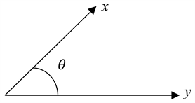
Project x onto y, to obtain ty:
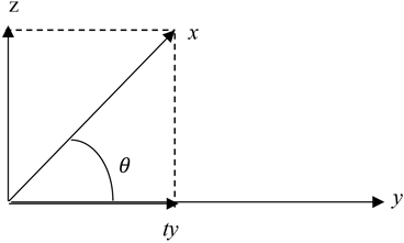
Then we have
Taking the inner product with y, we get
On the other hand,
If we equate the two formulas for t we get
We say that two vectors are orthogonal if
; this is equivalent to the angle between x and y being
. If
, then we will say that x and y form an acute angle; This is equivalent to
. If
, then we will say that x and y form an obtuse angle; this is equivalent to
. Non-zero vectors also define some useful geometric objects. Let
be non-zero. We may consider three sets that partition V:
The first set consists of the vectors that form an acute angle with v, the middle set is the hyperplane P orthogonal to Rv, and the last set consists of the vectors that form an obtuse angle with v. We refer to the first and last sets as the half-spaces defined by P. Of course, v lies in the first half-space. The formula for the reflection sv shows that
for x in V, so that S sends one half-space into the other half-space. Also, S acts by the identity on P. Multiplication by −1 also sends one half-space into the other half-space; however, while multiplication by −1 preserves P, it is not the identity on P.
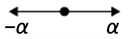
Example 5.7: A1: The only rank 1 root system is
with inner product
and roots
. Its Weyl group is given by
. We call this root system A1. This is the root system of sl2.
Example 5.8: [8]
: Take
with the usual inner product. Then
with the standard basis vectors is a root system. Note that this is
and therefore not irreducible. Here
(Figure 1).
: Let
. Then
. We call this root system
, it appears as the root system of
.
: Let
,
,
,
,
are short
roots,
long roots. Then W is the symmetry group of the square, i.e.
, the dihedral group of order 8. This is the root system of
and
.
: Also
appears as Weyl group of a root system, called
.
Example 5.9: Let V be a vector space over R with an inner product
. Let
and assume that x and y are both non-zero. The following are equivalent:
1) The vectors x and y are linearly dependent.
2) We have
.
3) The angle between x and y is 0 or π.
Proof. Let
be the angle between x and y. We have
Assume that
. Then
, and
, so that
. This implies that
or
.
Suppose that
. We have
It follows that
, so that x and y are linearly dependent.
Example 5.10: [6] Let V be a finite-dimensional vector space over R equipt with an inner product
, and let R be a root system in V. Let
, and assume that
and
. Let
be the angle between α and β. Exactly one of the following possibilities holds Figure 2.
Proof. By the assumption
. We have
, so that
![]()
Figure 2. Possible angles and ratio of norms between pairs of roots.
we have that
and
are integers, and we have
. These facts imply that the possibilities for
and
are as in the table.
Assume first that
. From above,
.
It follows that
, so that
.
Assume next that
. Now
so that
is positive and
This yields the
column. Finally,
so that
This gives the
column.
Definition 5.11: R is simply laced if all the roots are of the same length (e.g.
,
,
, not
,
).
Example 5.12: [6] Let
equipt with the usual inner product
, and let R be a root system in V. Let
be the length of the shortest root in R. Let S be the set of pairs
of non-colinear roots such that
and the angle θ between α and β is obtuse, and β is to the left of α. The set S is non-empty.
Fix a pair
in S such that θ is maximal. Then
1) (
root system) If
(so that
) then R, α, and β are as follows Figure 3:
2) (
root system) If
(so that
) then R, α, and β are as follows Figure 4:
3) (
root system) If
(so that
) then R, α, and β are as follows Figure 5:
Proof. Let
be a pair of non-colinear roots in R such that
such a pair must exist because R contains a basis which includes α. If the angle between α and β is acute, then the angle between α and −β is obtuse. Thus, there exists a pair of roots
in R such that
and the angle between αand β is obtuse. If β is the right of α, then −β forms an acute angle with and is to the left of α; in this case,
forms an obtuse angle with α and
is to the left of β. It follows that S is non-empty.
Assume that
so that
. It follows that
. By geometry,
. It follows that R contains the vectors in 1. Assume that R contains a root other than
. We see that must lie halfway between two adjacent roots from
. This implies that
is not maximal, a contradiction.
Assume that
so that
. We have
. It follows that R contains
so that R contains the vectors in 2. Assume that R contains a root
other than
Then
must make an angle strictly less than 30° with one of
Assume that
so that
. We have
. By geometry, the angle between
and
is 30°. By geometry, the angle between
and
is 120°. By
. It now follows that R contains the vectors in 3. Assume that R contains a vector
other than
. Then must make an angle strictly less than 30° with one of
.
6. The Future Perspective of This Paper
The future perspective of this paper is to support me in writing a book on Lie algebras. In addition, it is possible to do work for each of the titles in the paper. Each of the titles creates an opportunity for research, because from each title, there are many opportunities for research and to write. My future is to work on comparing many facts and applying leftist algebras in everyday life. Comparing all these disciplines with left algebras, we see closely connectivity and the need to apply and use it properly.
NOTES
1Let L be a Lie algebra over F, let V be a finite-dimensional F-vector space, and let
be a representation. Define
by
for
.