Received 11 November 2015; accepted 8 December 2015; published 11 December 2015

1. Introduction
Usually harmonic functions are defined by Laplace operator , where
 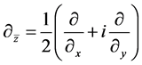 is the Cauchy-Riemann operator and
  is the adjoint operator of C-R operator. By iterating the
Laplace operator, one can define the so-called polyharmonic functions by  [1] . In [2] , Goursat obtained his decomposition formula, in [3] , Vekua developed one method to construct an approximative solution of the biharmonic Dirichlet problem in a simply connected domain. In recent years, the study of explicit solution of BVPS (boundary value problems) has undergone a new phase of development [4] - [6] . There are Dirichlet, Neumann and Robin boundary value problems in regular domain (in the disc [4] ; and in the upper half plane [5] ) and in irregular domains (Lipschitz domains [6] ). Although, there are many marked works about the BVPS, few of them give a certain estimate about the uniqueness of the solution. Thus, the purpose of this article is devoted to solving the unique solution of the following polyharmonic Dirichlet problems (for short, PHD) for
  data in the upper half plane, H, i.e.
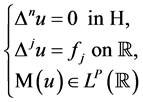 (1.1)
(1.1)
with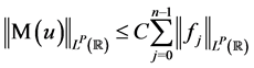 , where
  is the Laplacian, and
  is the real axis,
  for some
suitable ,
,  ,
,  ,
,  is the non-tangential maximal function of u, which is defined by
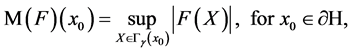
where ![]() is the non-tangential approach region, viz.,
is the non-tangential approach region, viz.,
![]()
where![]() .
.
It is clear that all the boundary data in BVPs (1.1) are non-tangential.
2. Preliminary and Some Lemmas
Definition 2.1. If a real valued function ![]() satisfies the equation
satisfies the equation![]() , in D, then f is called an n-harmonic function in D, concisely, a polyharmonic function.
, in D, then f is called an n-harmonic function in D, concisely, a polyharmonic function.
We use the notation ![]() denoting the set of polyharmonic function of order n in D. Especially,
denoting the set of polyharmonic function of order n in D. Especially, ![]() is the set of all harmonic functions in D.
is the set of all harmonic functions in D.
Lemma 2.2. [7] Let D be a simply connected (bounded or unbounded) domain in the complex plane with smooth boundary![]() . If
. If![]() , then for any
, then for any![]() , there exist functions
, there exist functions![]() ,
, ![]() such that
such that
![]() (2.1)
(2.1)
where ![]() denotes the real part. The above decomposition expression of f is unique in the sense of the equi- valence relation
denotes the real part. The above decomposition expression of f is unique in the sense of the equi- valence relation![]() , more precisely,
, more precisely, ![]() for
for![]() .
.
Corollary 2.3. If the sequence of functions ![]() defined in D satisfy
defined in D satisfy
(1)![]() ;
;
(2) ![]() in D for
in D for![]() .
.
Then ![]() for
for![]() , and
, and
![]() (2.2)
(2.2)
where ![]() is the analytic jth decomposition component of the n-harmonic function
is the analytic jth decomposition component of the n-harmonic function![]() . It must be noted that (2.2) holds in the sense of the equivalence relation
. It must be noted that (2.2) holds in the sense of the equivalence relation![]() .
.
Definition 2.4. A sequence of real-valued functions of two variables ![]() defined on
defined on ![]() is called a sequence of higher order Poisson kernels, more precisely,
is called a sequence of higher order Poisson kernels, more precisely, ![]() is called the nth order Poisson kernel, if they satisfy the following conditions.
is called the nth order Poisson kernel, if they satisfy the following conditions.
(1) For all![]() ;
; ![]() with any fixed
with any fixed![]() ; and
; and![]() , with any fixed
, with any fixed![]() , and the non-tangential boundary value
, and the non-tangential boundary value
![]()
exists for all t and![]() ;
; ![]() can be continuously extended to
can be continuously extended to ![]() for any fixed
for any fixed![]() ;
;
(2) ![]() and
and ![]() and
and![]() , and for any
, and for any ![]()
![]()
uniformly on ![]() whenever
whenever![]() , where
, where ![]() is any compact set in
is any compact set in![]() , M, T are positive constants depending only on
, M, T are positive constants depending only on ![]() and n;
and n;
(3) ![]() and
and ![]() for
for![]() ;
;
(4)![]() , a.e., for any
, a.e., for any![]() ;
;
(5)![]() , for any
, for any![]() ,
,
where all limits are non-tangential.
Definition 2.5. Let D be a simply connected (bounded or unbounded) domain in the plane with smooth boundary![]() , and
, and ![]() denote the set of all analytic functions in D. If f is a continuous function defined on
denote the set of all analytic functions in D. If f is a continuous function defined on ![]() satisfying
satisfying ![]() for any fixed
for any fixed![]() , and
, and![]() ,
, ![]() , for any fixed
, for any fixed![]() , then f is called
, then f is called ![]() on
on ![]() and this is noted by
and this is noted by![]() .
.
Lemma 2.6. [8] If ![]() is a sequence of higher order Poisson kernels defined on
is a sequence of higher order Poisson kernels defined on![]() , i.e.,
, i.e.,
![]() fulfills the aforementioned properties 1 - 5 in Definition 2.4, then, for
fulfills the aforementioned properties 1 - 5 in Definition 2.4, then, for![]() , there exist functions
, there exist functions
![]() defined on
defined on ![]() such that
such that
![]() (2.3)
(2.3)
with
![]() (2.4)
(2.4)
for ![]()
![]() (2.5)
(2.5)
for ![]() with respect to
with respect to ![]() and
and
![]() (2.6)
(2.6)
Moreover,
![]() (2.7)
(2.7)
is the classical Poisson kernel for the upper half plane. All of the above![]() , the non- tangential boundary value
, the non- tangential boundary value
![]() (2.8)
(2.8)
exists on![]() , except
, except ![]() and
and ![]() for any fixed
for any fixed![]() . We can further show that
. We can further show that ![]()
can be continuously extended to ![]() for any fixed
for any fixed![]() , and
, and
![]() (2.9)
(2.9)
uniformly on ![]() whenever
whenever ![]() which is any compact set in
which is any compact set in![]() , where M, T are positive constants depending only on
, where M, T are positive constants depending only on![]() .
.
Moreover,
![]() (2.10)
(2.10)
for any ![]() and
and![]() .
.
Remark 2.7. Lemma 2.6 provides a algorithm to obtain all explicit expressions of higher order Poisson kernels appeared in [8] .
3. Homogeneous PHD Problem in the Upper Half Plane
In order to solve the homogeneous PHD problems (1.1) and get the uniqueness of its solution, we need the following lemmas.
Lemma 3.1. [8] Let D be a simply connected unbounded domain in the plane with smooth boundless boundary![]() . If
. If ![]() and there exists
and there exists![]() , such that
, such that
![]() (3.1)
(3.1)
uniformly on ![]() whenever
whenever ![]() which is any compact set in D, where M, T, are positive constants depending only on
which is any compact set in D, where M, T, are positive constants depending only on![]() . Then
. Then
![]() .
.
Lemma 3.2. [8] Let ![]() be the sequence of higher order Poisson kernels defined on
be the sequence of higher order Poisson kernels defined on![]() , then
, then
for any ![]() and
and![]() ,
,
![]() . (3.3)
. (3.3)
Lemma 3.3. [9] Let![]() ,
, ![]() , and
, and ![]() be the Poisson integral of f (in our notations,
be the Poisson integral of f (in our notations,
![]() ,
,![]() ), then
), then
![]() (3.4)
(3.4)
where ![]() is the cone in
is the cone in ![]() with the vertex at
with the vertex at ![]() and the aperture
and the aperture![]() ,
, ![]() ,
,![]() ;
; ![]() is a positive constant depending only on
is a positive constant depending only on![]() ,
, ![]() is the non-tangential maximal function, and
is the non-tangential maximal function, and ![]() is the standard Hardy-Littlewood maximal function defined by
is the standard Hardy-Littlewood maximal function defined by
![]() (3.5)
(3.5)
Lemma 3.4. (Hardy-Littlewood maximal theorem, see [10] ) Let![]() ,
, ![]() , then
, then ![]() is finite almost everywhere on
is finite almost everywhere on![]() . Moreover,
. Moreover,
(1) If![]() , then
, then ![]() is in
is in![]() , more precisely
, more precisely
![]() (3.6)
(3.6)
(2) If![]() ,
, ![]() , then
, then
![]() (3.7)
(3.7)
where ![]() is a constant depending only on p.
is a constant depending only on p.
Corollary 3.5. ![]() for any
for any ![]() with
with![]() , where
, where ![]() is a constant depending only on
is a constant depending only on![]() . Moreover,
. Moreover,
![]() (3.8)
(3.8)
for any![]() , and for any
, and for any![]() ,
, ![]() ,
, ![]() is finite almost everywhere on
is finite almost everywhere on![]() ,
, ![]() is a positive constant depending only on
is a positive constant depending only on![]() .
.
Theorem 1. Let ![]() be the sequence of higher order Poisson kernels defined on
be the sequence of higher order Poisson kernels defined on![]() , then for any
, then for any![]() ,
,
![]() (3.9)
(3.9)
is the unique solution of PHD problem (1.1)
Proof. Since the higher order Poisson kernels possess the inductive property as stated in Definition 2.4. Act on the two sides of (3.9) with the polyharmonic operator![]() ,
,![]() . We have
. We have
![]() (3.10)
(3.10)
since the Laplace operator is![]() . Thus, for
. Thus, for ![]() on
on![]() ,
,
![]() (3.11)
(3.11)
follow from Lemma 2.6 and the nice property of G, i.e.,
![]() (3.12)
(3.12)
for any![]() .
.
Similarly, letting the polyharmonic operator ![]() act on the two sides of (3.9), we have
act on the two sides of (3.9), we have ![]() for any
for any![]() . Thus (3.9) is a solution of the PHD problem (1.1).
. Thus (3.9) is a solution of the PHD problem (1.1).
Next we turn to the estimate and uniqueness of the solution. By Definition 2.4 and Corollary 3.5, we have
![]()
As discussed above, the uniqueness of solution follows.
4. Inhomogeneous PHD Problem in the Upper Plane
Due to the limited knowledge of the author, at this section, we only consider the bounded domain D for in- homogeneous PHD problem in the upper half-plane, i.e.
![]() (4.1)
(4.1)
where![]() , such that, for some
, such that, for some![]() ,
, ![]() , as
, as ![]() and
and ![]() for some suitable
for some suitable![]() . In order to solve the inhomogeneous PHD problem (4.1), we need the higher order Pompeiu operators which are higher order analogues of the classical Pompeiu operators.
. In order to solve the inhomogeneous PHD problem (4.1), we need the higher order Pompeiu operators which are higher order analogues of the classical Pompeiu operators.
Definition 4.1. [11] Let kernels
![]() (4.2)
(4.2)
where m and n are integer, with ![]() but
but![]() . Then, we formally define operators
. Then, we formally define operators![]() , acting on suitable complex valued function w defined in D, a domain in the plane, according to
, acting on suitable complex valued function w defined in D, a domain in the plane, according to
![]() (4.3)
(4.3)
The following properties of ![]() are needed in the sequel. They are partial results from [11] .
are needed in the sequel. They are partial results from [11] .
Lemma 4.2. Assume![]() , and let w be a complex valued function in
, and let w be a complex valued function in ![]() such that for some
such that for some![]() ,
,
![]()
Then, the integral ![]() converges absolutely for almost all z in
converges absolutely for almost all z in ![]() and, provides that p satisfies con- ditions,
and, provides that p satisfies con- ditions,
![]()
![]() .
.
Proof. See Corollary 4.6 in [11] .
Lemma 4.3. Assume![]() , and let w be a measurazble complex valued function in
, and let w be a measurazble complex valued function in ![]() such that for some
such that for some![]() ,
,
![]() (4.4)
(4.4)
(a) If ![]() and
and![]() , then in the sense of Sobolev derivatives in the entire plane
, then in the sense of Sobolev derivatives in the entire plane![]() ,
,
![]() (4.5)
(4.5)
![]() (4.6)
(4.6)
(b) If ![]() and
and ![]() for some
for some![]() , then (4.5) and (4.6) again hold in the sense of Sobolev derivatives in
, then (4.5) and (4.6) again hold in the sense of Sobolev derivatives in![]() ; moreover, the formulas
; moreover, the formulas
![]() (4.7)
(4.7)
are valid in ![]() even in the case of
even in the case of![]() .
.
Proof. See Corollary 5.4 in [11] .
Theorem 2. The problem of (4.1) is solvable and its unique solution is
![]() (4.8)
(4.8)
where ![]() and
and ![]() are the higher order Pompeiu operators,
are the higher order Pompeiu operators, ![]() and
and ![]() are the former n higher order Poisson kernel functions.
are the former n higher order Poisson kernel functions.
Proof. Through Lemma 4.2 and Lemma 4.3, we get
![]() (4.9)
(4.9)
in the Sobolev sense. Moreover,
![]() . (4.10)
. (4.10)
Noting (4.9) we know that ![]() is a week solution of the inhomogeneous equation
is a week solution of the inhomogeneous equation
![]()
and for some
![]() (4.11)
(4.11)
By the aforementioned, the problem (4.1) is equivalent to the PHD problem of simplified form
![]()
So, through Theorem 1 as well as the estimate of the solution, we complete the proof of Theorem 2.