1. Introduction
In this paper,  is assumed to be a filtered probability space where
  is a filtration satisfying
  for all
 , the usual condition of right continuity and completeness. The random movement of
  risky assets in the market is modeled via cadlag, nonnegative stochastic processes
 , where
 . We assume that all wealth processes are discounted by another special asset which is considered a baseline. In the market described above, economic agents can trade in order to reallocate their wealth.
Consider a simple predictable process
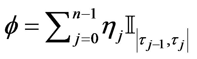 .
.
where , and for all
 ,
,  is a finite stopping time and
  is
is  -measurable.
Each ,
,  , is an instance when some give economic agent may trade in the market, then,
  is the number of unit from the ith risky assets that the agent will hold in the trading interval
 . This form of trading is called simple, as it comprises of finite number of buy-and-hold strategies, in contrast to continuous trading where one is able to change the position of the assets in a continuous fashion. The last form of trading is only theoretical value, since it cannot be implemented in reality, even if one ignores market frictions.
Starting from initial capital  and following the strategy described by the simple predictable process
 , the agent’s discounted process is given by
 .
.
where ,
, 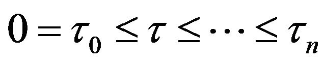 are a.s. finite stoping times with respect to
  and the
  are
are  -measurable real random variables. Note that the trader is allowed to trade on an infinite time horizon, because we do not restrict to bounded stoping times for the re-allocation of the capital. Of course trading on a finite time horizon [0, T] is covered by switching to the process
 .
.
Theorem 1.1. [1,2] A real valued, cadlag, adapted process  the following are equivalent:
1) X is a good integrator.
2) X may be decomposed as , where
  is a local martingale and
  is an adapted process of finite variation.
Defination 1.1. [1,3] A real valued, cadlag, adapted process  allows for A Free Lunch With Vanishing Risk for simple integrands if there is a sequence
  of simple integrands such that for
 ,
,
 .
.
and

In contrast, X therefore admits No Free Lunch With Vanishing Risk (NFLVR) for simple integrands if for every sequence  satisfying (VR) we have
(NFL)  in probability.
A free lunch with vanishing risk (FLVR) for simple integrands indicates that S allows for a sequence of trading schemes , each
  involving only finitely many rebalancing of the portfolio, such that the losses tend to Zero in the sense that of (VR) ,while the terminal gains (FL) remain substantial as n goes to infinity. It is important to note that the condition (VR) of vanishing risk pertains the maximal losses of the trading strategy
  during the entire interval [0,T]: if the left hand side of (VR) equals
  this implies that, with probability one, the strategy
  never, i.e. for not
 , cause an accumulated loss of more than
 .
.
Resently, it has been argued that existence of an Equivalent Martingale Measure(EMM) is not necessary for viability of the market; to see this effect, see [4-6]. In [7], the concept of strictly positive supermartingale deflator which is weaker than the existence of an EMM, that allows for consistent theory to be developed.In this paper, we investigate the relation between the no free lunch with vanishing risk property for simple integands and the semimartingale property.
Theorem 1.2. [1,8] Let  be a real-valued, cadlag, locally bounded process based on and adepted to a filtered probability space
 . If S satisfies the condition of no free lunch with vanishing risk (NFLVR) for simple integrands then S is a semimartingale.
Theorem 1.3. For a locally bounded, adopted, cadlag process X the following are equivalent 1) X satisfies NFLVR + LI(little Investment)
2) X is a classical semimartingale.
Theorem 1.4. For an adapted cadlag process X the following are equivalent.
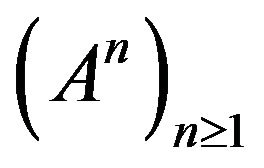
1) For all sequences  of simple predictable processesa)
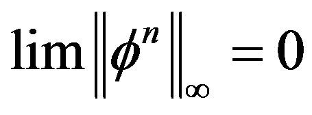
b) 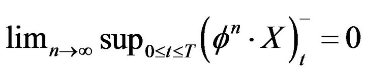
together imply 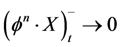 in probability.
2) X is a classical semimartingale.
Proposition 1.5. Let  be cadlag and adapted, with X0 and such that
  and X satisfies NFLVR + LI For all
  there is
  and a sequence of stopping times
  such that, for all n 1)
  takes values in
 .
.
2) .
.
3) The stopped processes  and
and  satisfyfor all n,
 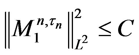 and
and
Lemma 1.6. Under the assumptions as in the proposition above with
 the sequence
  is bounded in probability.
Proof. For all n, let
a simple predictable process, then 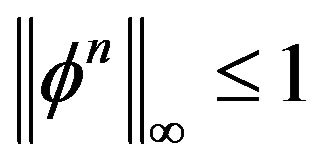 since
since 
since X satisfies NFLVR + LI,  is bounded in
 .
. 
For  define a sequence of stopping times
 .
.
Given  there is
  such that
Lemma 1.7. Under the same assumptions as in Proposition 1.5 the stopped martingales  satisfy
 .
.
Proof. For  and
and , since the
  are predictable and the
  are martingales,
we write 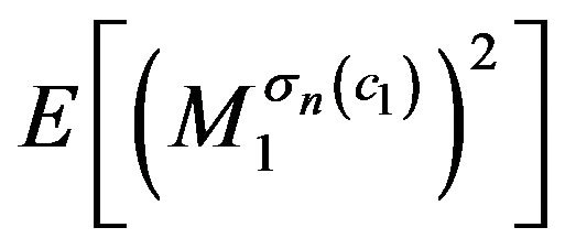 as a telescoping series and simplifying to get

Lemma 1.8. Let
 .
.
Under the assumption of Proposition 1.5 the sequence  is bounded in probability.
Proof. Assume for contradiction that  is not bounded in probability. Then there is
  such that for all k there is
  such that
  For
For  define
and
 .
.
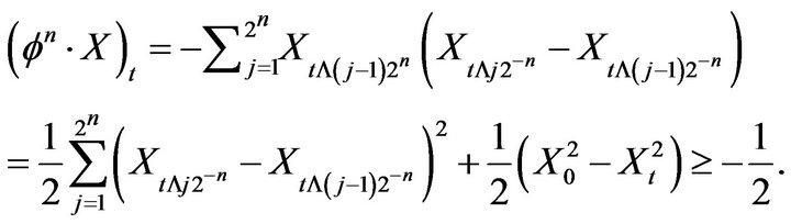
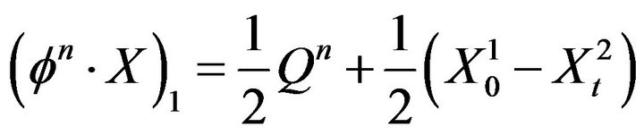
Then  and
and
and at time t = 1 we have
 .
.
But the second summand is bounded in L2, so we conclude that  is not bounded in probability.
We defined a sequence of stopping times
 .
.
Because
by Doob’s sub-martingale in-equality,(see [9,10])
 is bounded in probability. Therefore there is
  such that
 . Note that
  is uniformly bounded below by
 . We claim
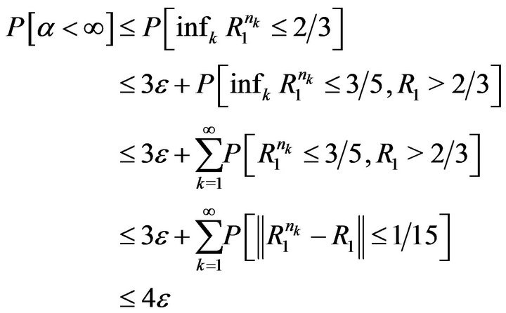
  is not bounded in probability. Indeed, for any n and any k,

Since , the probability of the other event is at least
 . This gives the desired contradiction because it is now easy to construct a FLVR + LI.
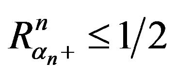
Proof of Proposition 1.5: Defined a sequence of stopping times
 .
.
By Lemma 1.8 there is c2 such that . Take
  and
and 
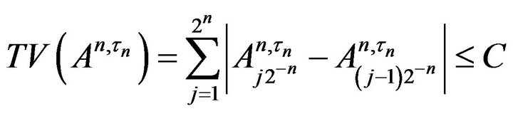
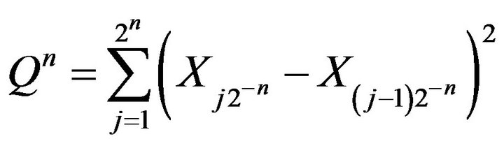
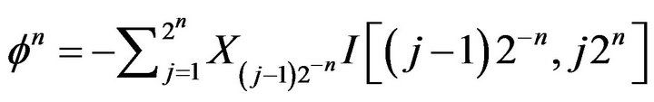
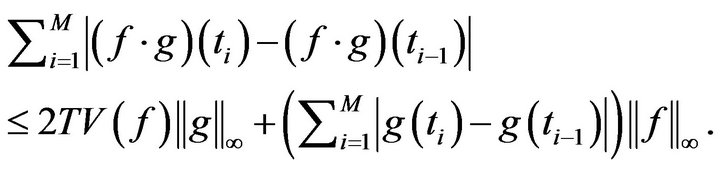
Lemma 1.9. [11]. Let  be measurable functions, where f is left continuous and takes finitely many values. Say
 . Define
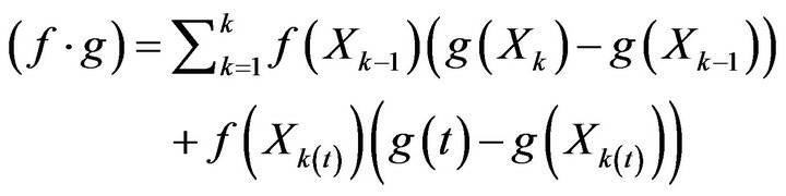
where 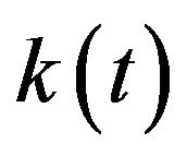 is the biggest of the k such that Xk less than or equal to t. Then for all partition
 ,
,
Proposition 2.0. Let 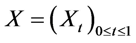 be cadlag and adopted, with
  and such that
  and X satisfies NFLVR + LI. For all
  there is C and a
  valued stopping time
  such that
 and sequence
  and
and  of continuous time cadlag processes such that for all n1)
2) 
3)  is a martingale with
4) 
Proof. Let  be given. Let C,
  ,
,  , and
, and  be as in proposition 1.5. Extended
 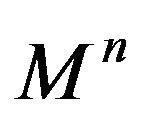 and
and 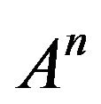 to all
  by defining
 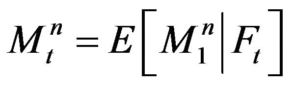 and
and
 . Not that the extended
  is no longer predictable, and currently we only have control of the total variation of
  over
over , i.e.

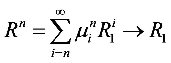
Notice that, for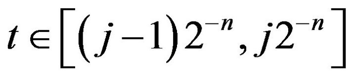 ,
,
From this and  it follow that
 , so
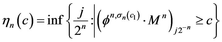
, so . How do we fine the limit of the sequence of stopping times
 ? The trick is to define
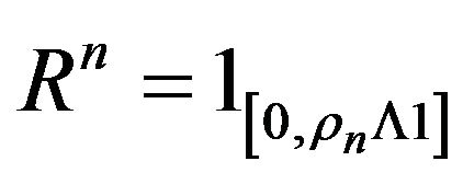 , a simple predicator process, and note that stopping at
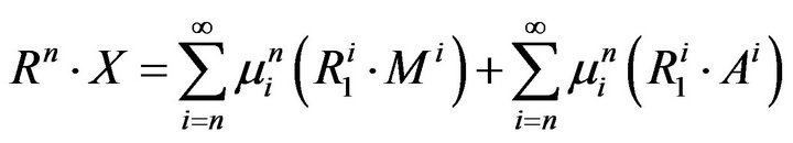
  is like integrating Rn, i.e.
 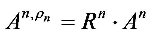 and
and . We have that
 .
.
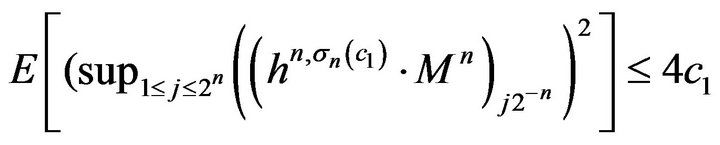
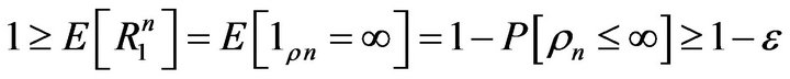
Apply Komlos’ Lemma to obtain convex weights  such that
a.s as  By the dominated convergence theorem,
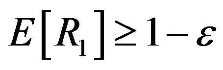 . Observe that
Define . Each
  is left continuous, decreasing process. In particular,
 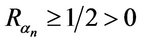 , so we can divide by this quantity. We claim that
 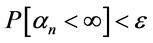 . In deed, on the event
 ,
, 
 so
so

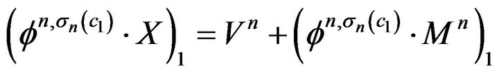
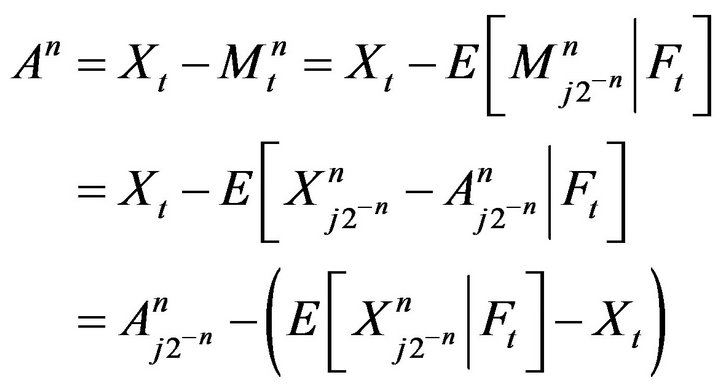
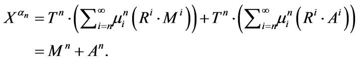
Define new processes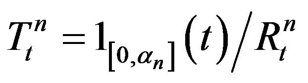 . Then
 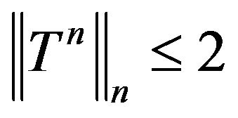 and
and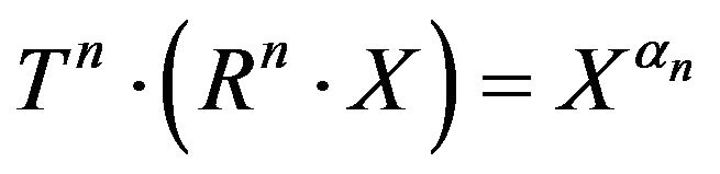 . Thus we define Mn and An by
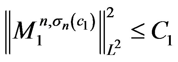
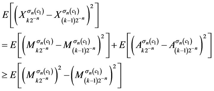
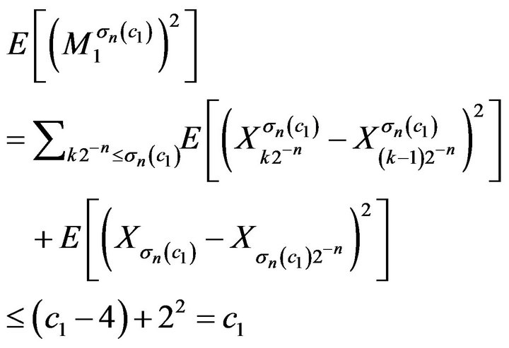
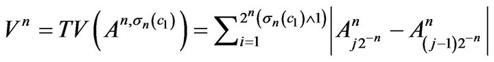
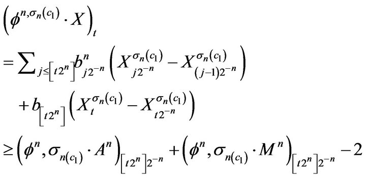
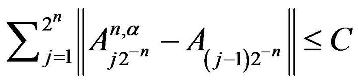
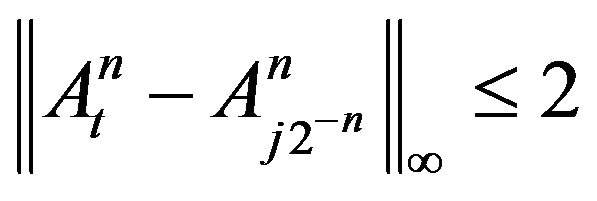
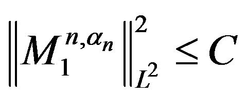
The total variation of  over
over  is bounded by 3. By Lemma 1.9,

That 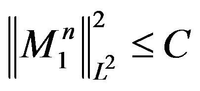 follows from the fact that
 . To finish the proof, we show that there is a subsequence
  such that
 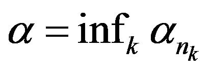 satisfies
 . We know
  because
 . Since
  a.s there is a subsequence such that
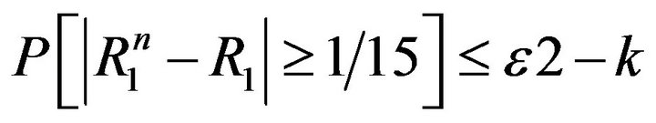 . Finally,
Therefore ,
,  and
and  have the desired properties.
Proof of the Main Theorems Proof of Theorem 1.3. We may assume the hypothesis of proposition. Let  and take C,
  ,
,  ,
,  as in proposition. Apply komlos lemma to find convex weights
  such that


for all , where the convergence is a.s. For all n,
 so the total variation of A over D is bounded by C. Further, we have
 . A is a cadlag on D, so define it on all of [0,1] to make it cadlag. M is
  martingale so it has a cadlag modification. Since
  and
and  was arbitrary, and the class of classical semimartingales is local, X must be a classical semimartingale.
Proof of Theorem 1.4. We no longer assume that X is locally bounded. The trick is to leverage the result for locally bounded processes by subtracting the big jump from X. Assume without loss of generality that  and defined
 . Then X = X − J is an adopted, cadlag locally bounded process. We will show that theorem 1.4 for X implies NFLVR + LI for X, so that we may apply theorem 1.3 to X. Then since J is finite variation, this will then imply X is a classical semimartingale .
Suppose 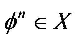 are such that
  and
and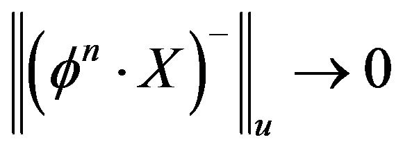 . We need to prove that
 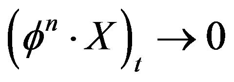 in probability . First we will show that
 .
.
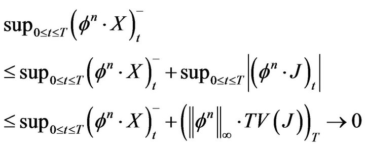
by the assumptions on 
By (1), 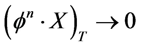 in probability. Since
 in probability, we conclude that
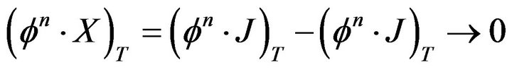
in probability. Therefore X satisfies NFLVR + LI. 
NOTES