A Two-Step Growth Curve: Approach to the von Bertalanffy and Gompertz Equations ()
Received 20 February 2016; accepted 12 April 2016; published 15 April 2016

1. Introduction
Selecting a curve to model individual growth for marine invertebrates can be difficult because invertebrates exhibit a suite of complicated growth features [1] . Many invertebrates exhibit staged growth, for example crabs and lobsters molt their hard exoskeleton to permit growth [2] . Some invertebrates are thought to have continuous or indeterminate growth throughout their lives [3] . Growth during the juvenile stage may include a lag until some intermediate size is reached after which growth is maximized [4] . Somatic growth may slow when invertebrates mature and shift energy allocation to reproduction [5] [6] . Invertebrates can also shrink in size, restructuring calcium hard-parts such as sea urchin tests, and rough wave action can wear down mollusk shells out pacing slow growth in large adults. Invertebrates and some fishes do not appear to follow first order growth as suggested by traditional von Bertalanffy growth curves, so that new models have been proposed [7] - [9] . Furthermore, decisions regarding which growth models to use can have major impacts on predicted growth rates. For example, if 75% of adult size is a minimum legal size, the time to fishery estimated by the sigmoidal curve may be double that of the first order curve.
Due to these complications and the importance for modeling invertebrate growth, there has been disagreement in the modeling community as to the appropriateness of selecting a first order growth equation (e.g. von Bertalanffy) or a sigmoidal curve (e.g. Gompertz). Even with the von Bertalanffy model there have been calls for use of the three-parameter von Bertalanffy compared with the two-parameter model due to bias in estimates generated from the two parameter form [10] . It has been suggested that since some invertebrates continue to grow very slowly, models which approach a gradual linear increase may be best, a feature the von Bertalanffy model lacks. The von Bertalanffy function [11] , which is commonly used to model growth in fishes, has been shown to overestimate juvenile growth for invertebrates [4] [7] . Therefore, other models have been used such as the Gompertz model [12] - [15] and the Ricker family of curves [16] . Models such as the Tanaka function [17] and the Gaussian model [18] have also been used as they can accommodate some of the complications observed for invertebrate growth. The inverse logistic has been shown to perform best for some invertebrates [7] [8] and this type of model has the advantage of having low biological prediction error [19] . Growth can also be seasonal and there have been efforts to incorporate seasonality into growth models [15] [20] which require an increase in the number of parameters in the model [21] . Therefore, selecting an appropriate growth model is not a trivial task and selection has been shown to have an impact on fisheries model results impacting management decisions.
Fishery modeling efforts are sensitive to both growth model selection and growth parameters. Optimal fishing mortality rates (F) are heavily influenced by growth parameters. Calculating growth rates directly based on tag recapture or indirectly using size frequency methods can also lead to disparate results [22] . Selecting models or methods which overestimate growth can lead to fishing policies that are too liberal while underestimating growth can lead to conservative fishing policies. Excessive fishing compared to growth capacity can lead to overfishing and population collapse. Overly conservative fishing policies can hurt the economic viability of fisheries. Egg per recruit models, for example, have been shown to be sensitive to growth parameter estimates significantly changing EPR model projections [23] . Therefore, given the critical importance of growth parameter estimation a method that allows for flexibility in mapping a wide range of growth possibilities is needed.
To examine how different types of growth can be accommodated, we explored a novel method of visualizing and modeling growth using a simple two-step, three-stage growth model 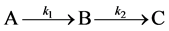 which may ameliorate some of the apparent contradictions reported for both increment data and growth modeling. We examine the rate equations which progress through three (or more) growth stages A, B, and C. These equations yield either a sigmoidal approach to the fully grown state if the growth rates k1 and k2 are similar, or to a first order von Bertalanffy curve if they are not. Finally, we show by allowing the growth rate ratio to vary with time that the result produces a growth surface over which the actual growth of an individual organism can be mapped. We emphasize that we are not proposing a new model to add to the vast collection of growth models being used already, but that we are showing how apparent contradictions in previous studies can be reconciled for organisms that grow by two or more stages since growth can be envisioned across a growth surface that encompasses a suite of growth trajectories (models).
2. Theory
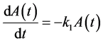
Growth studies often follow a conventional one-step model

which leads to the first order equation
 (1)
(1)
which yields
 (2)
(2)
A change of notation gives,
 (2a)
(2a)
where  denotes size and
  denotes the final size attained at a time substantially greater than the period of active growth (“infinite” time). This equation is commonly called the von Bertalanffy equation or Brody-von Bertalanffy equation [10] .
We seek to examine results from a sequential growth model which focuses on transitions between distinct stages. These stages may encompass radical metamorphosis (changes in body plan) or more subtle transitions from juvenile to reproductive adult which do not change outward appearance.
A sequential growth mechanism involving first order steps

follows the equations
 (3a)
(3a)
 (3b)
(3b)
and
 (3c)
(3c)
At time zero,

![]() and
and ![]()
From Equation 3(a),
![]()
where
![]()
as in Equation (1). The result for B ® C requires substituting for A(t) into the rate law of B(t)
![]()
A (no italic) identifies a stage A and italic ![]() represents the size of a potential growth function which is diminished when an individual progresses from stage A to growth stage B. In stage B the growing animal has a potential growth function of size
represents the size of a potential growth function which is diminished when an individual progresses from stage A to growth stage B. In stage B the growing animal has a potential growth function of size ![]() which is transformed into the size of the animal represented by
which is transformed into the size of the animal represented by ![]() at growth stage C. Using Laplace integral transforms [24] - [26] : see mathematical Appendix, one obtains
at growth stage C. Using Laplace integral transforms [24] - [26] : see mathematical Appendix, one obtains
![]()
At any time,
![]()
![]()
![]()
where n = k1 − k2.
3. Methods and Results
We shall maintain the distinction between growth of an animal and growth of a population. Here we consider animal growth and not population growth. We have expressions for transitions from stages A, to B, and B to C as a function of time t, A(t), B(t), and C(t) (Notice that ![]() is a parameter, not a variable). We can look at the effect of the two stage model on the growth curve in Figure 1.
is a parameter, not a variable). We can look at the effect of the two stage model on the growth curve in Figure 1.
One can look at the model from two sides, the two extreme cases, one in which ![]() and the other case where
and the other case where![]() . In the first extreme case, the transfer rate from stage 1 to stage 2 (from A to B) is large and the entire system rushes from A to B only to be detained by slow passage from B to C. In this case, the second transfer controls the total transfer and the second step is the rate controlling step. The rate of increase of C(t) (growth) is controlled entirely by the second step rate constant
. In the first extreme case, the transfer rate from stage 1 to stage 2 (from A to B) is large and the entire system rushes from A to B only to be detained by slow passage from B to C. In this case, the second transfer controls the total transfer and the second step is the rate controlling step. The rate of increase of C(t) (growth) is controlled entirely by the second step rate constant ![]() and the rate equation is a first order von Bertalanffy type equation.
and the rate equation is a first order von Bertalanffy type equation.
In the second extreme case, the rate controlling step is the first transfer, which is slow from A to B followed by a fast transfer from B to C. The growing animal moves through the transition from A to B slowly but the magnitude of the potential growth function B(t) is quickly drawn off to growth stage C. B(t) never becomes very large (see Mathematical Supplement Figure S1). The rate equation is again first order but it has a different rate constant![]() . Only when the two rate constants k1 and k2 are fairly close to one another does one see the sigmoidal nature of the two stage process in Table 1.
. Only when the two rate constants k1 and k2 are fairly close to one another does one see the sigmoidal nature of the two stage process in Table 1.
An interesting point arises when we take the growth surface through the minimum at![]() . The surface is not defined because k1/k2 − k1 has zero in the denominator. Also
. The surface is not defined because k1/k2 − k1 has zero in the denominator. Also ![]() is zero. This should not cause concern because the surface is reinstated on the negative side of the t = 0 axis. The denominator in k1/k2 − k1 changes sign when k1 becomes dominant but the sign of
is zero. This should not cause concern because the surface is reinstated on the negative side of the t = 0 axis. The denominator in k1/k2 − k1 changes sign when k1 becomes dominant but the sign of ![]() also changes so the surface is
also changes so the surface is
![]()
Figure 1. Two views of the growth model surface. The views differ in the range of the n = k1 − k2 or n = k2 − k1 axis which varies from 0 to 1000 on the left and 0 to 1.4 on the right. For two-stage growth over a range of n = large, (a) there is only first order growth but when n = small, (b) the same two-stage mechanism predicts sigmoidal growth of size C(t).
![]()
Table 1. Parameters in the growth model.
reinstated on the negative side of k1/k2 − k1.
B(t) has a maximum at the inflection point of the function C(t) = f(t). It can be related to the distance between the actual curve at the inflection point and the curve that would be found if von Bertalanffy kinetics had been followed. The ratio of k1/k2 can be estimated from the distance between the actual curve and the experimental curve had the first order function been followed. As the distance between the actual curve and the hypothetical first order curve approaches zero, the ratio approaches 1. Practical use of this relationship would require very accurate experimental data.
4. Discussion
In this paper, we present a multistage growth model which shows the relationship between a suite of linear and non-linear growth curves across a growth surface used to model individual growth. We show that the rates of growth between stages determine the growth trajectory that can be described as a family of curves with the first order curve or the sigmoidal curve as limits. Depending on the difference in the values of the growth rate constants (n = k2 − k1), the growth trajectory follows a first order or sigmoidal portion of the growth surface in Figure 1 with the slower growth rate as the rate limiting step.
When both growth rates k1 and k2 are similar, the final growth trajectory follows a sigmoidal curve and when they differ it follows a first order trajectory (1 − e−kt). Because growth from stage A to growth stage C can be represented as a surface, we envision growth curves that vary across the entire surface such that size is a function of two variables C(t) = f (n, t). With this model, we see that individual growth can be described as a first order curve or as sigmoidal curve depending on the difference in the values of k. This allows for an infinite number of combinations and variations in individual growth across the growth surface as may occur with marine invertebrates.
The three stage model can be expanded to stages beyond C as a simple extension of the present model to stages D, E, and so on. Within a two (or more) stage growth model, it is possible for different research groups to report (correctly) different growth curves for similar populations. Different portions of the growth surface dominate during different life history stages. Likewise, different portions of the curve describe growth under different environmental conditions. For example, growth in red abalone slows during warm water periods such as El Niño events when kelp resources are scarce [27] . In addition, growth is often seasonal such that animals grow more during some parts of the year than others [21] [28] .
There are many factors which may influence growth in addition to environmental factors. Selection, either natural or artificial, may act as a force favoring fast or slow growth. Variation in abalone size plays a role in abalone culture facilities for aquaculture (R. Fields pers. comm.) and conservation. Small size adults may dominate especially in heavily fished populations [29] . Queen conch, for example, is fished in the Caribbean and at some sites there are only small adults with thick shells called “sambas” [30] . Similarly, in the abalone fishery in Australia differences in growth are found in abalone leading to protected reefs with small adults known as “short beds” just under the minimum legal size [31] . Regional growth rates may also differ such as with Geoduck, Panopea globose, in Mexico with important implications for management [32] . Adults that reach a small final size may have different growth rates compared to those which reach larger final sizes [33] .
Invertebrates tend to have high levels of individual variation in both growth rate and final size. Final size, C∞ in the von Bertalanffy or Gompertz model can be thought of as a distribution of maximum lengths since populations are filled with adults of varying sizes [33] . Model final size can also be thought of as the “most probable” value in a distribution of actual final sizes [7] . Differences in the shape of the growth model have been accommodated in the earlier Richards family of curves [34] by the addition of a poorly defined “shape parameter” which when it = 1 gives the logistic curve (sigmoidal) and when it = −1 gives the von Bertalanffy (first order).
![]()
Figure 2. Two-stage growth curve for n large (a) and n small 1 (b) (see Mathematical Supplement below). Units of k are reciprocal time, typically years. Numerical labeling of the axes, in Figure 2, is arbitrary because we can choose any unit for size or time but note the change in scale for the time axis. We have chosen the size at “infinite time” to be 1.0 which makes the potential for growth also 1.0 arbitrary units at t0 = 0.
In this work, we show that in a two stage model, shape is controlled by the well defined ratio k1/k2 − k1. This ratio is an improvement over previous methods as it explicitly shows what stage is controlling the growth trajectory.
The trajectory across the surface defines a path of the probability maximum over points on the growth surface. Fast, slow and negative growth can be accommodated by the growth surface in Figure 2.
In a two stage model, the growth rate C(t) = f(n, t), on the surface represents all possible curves. By selecting one growth curve it is possible to specify the curve which represents the most probable growth curve. There are many ways growth may vary because individual trajectories can move along the k1/k2 − k1 surface in any direction. This flexible growth surface allows for visualization of all possible growth trajectories and will be useful in modeling growth in animals with complex life histories, staged growth and even negative growth. The well defined parameters will allow for better estimates of growth for use in fishery and population models.
Acknowledgements
We thank the Whiteley Center at Friday Harbor Laboratories (University of Washington) for creating a space for us to think about growth modeling. We thank K. Rogers for facilitating this work. This work was funded in part by a grant to LRB from the SeaDoc Society, Wildlife Health Center at the University of California, Davis. This research was supported by a NOAA Section 6 grant to the California Department of Fish and Wildlife NA10NMF4720024 and to its partner the University of California, Davis at the Karen C. Dreyer Wildlife Health Center (P1570004). This work benefited from Tully’s coffee cups and fried oysters (Friday’s Crab Shack, Friday Harbor, WA). The first author LRB is supported by the California Department of Fish and Wildlife. This is a contribution of the Bodega Marine Laboratory at the University of California, Davis.
Mathematical Supplement
S.1. The Laplace Integral Transform
The Laplace Transform ![]() is defined
is defined
![]()
Its usefulness is in stepping down from a more difficult problem to an easier one, for example stepping down from ![]() to
to![]() . In our particular application,
. In our particular application,
![]()
Integration by parts gives
![]()
which is the simplification we sought.
S.2. Application
We wish to solve
![]()
Find ![]() of both sides
of both sides
![]()
An initial condition was that ![]()
![]()
![]()
![]()
Figure S1. Replicates Figure 2(b) text but it shows A(t), B(t), and C(t).
![]()
Figure S2. B(t) is just visible (bottom right).
![]()
Figure S3. B(t) goes negative but A(t) and C(t) are normal [see text].
Now taking the inverse transforms
![]()
There is no reason to believe that the rate parameter governing any stage transition will be constant (deterministic). For this reason we propose a growth surface over which an animal or population growth mean may wander during the growth process (Figure S1-S3).