Expansion by Laguerre Function for Wave Diffraction around an Infinite Cylinder ()
1. Introduction
The Rankine source panel method needs a large number of panels due to panelizing the free surface as well as a damping zone avoiding the reflected wave from the sides of a numerical fluid domain. So a control surface can be introduced to divide the fluid domain into two subdomains by a control surface. This surface separates the problem into two problems: 1) the interior one in which the ship is of any form, the Green function is Rankine source Green function; 2) the exterior one in which the shape of the control surface is known and velocity potential is assumed to be known. It brings two important benefits: area to be discretized becomes smaller; no need to introduce the damping zone [1].
A circular cylinder is adopted as control surface. The vertical variation of water diffraction wave is assumed to be the form  which is represented by a series of Laguerre functions
 . Laguerre functions
  which are defined by Laguerre polynomials
  are a system of orthogonal functions on the interval [0, ¥] [2]. It plays an important role in approximation and interpolation.
The purpose of this paper is to validate the accuracy and convergence of Laguerre series and approximate the vertical velocity potential f on an infinite cylinder generated by a body. Section 2 introduces basis of Laguerre functions. Section 3 provides an analytical method to approximate the function 1/(1 + z)n and the velocity potential f by Laguerre functions. Section 4 uses some examples to investigate the convergence and accuracy of the method, and compares the result of Compass-Walcs-Basic.
2. The Basis of Laguerre Function
2.1. Laguerre Polynomials
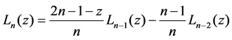
The Laguerre polynomials are defined by the three-term recurrence relation
 (1)
(1)
 (2)
(2)
 (3)
(3)
 is called nth degree Laguerre polynomial [3].
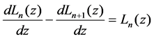
The Laguerre polynomials have some useful relations
 (4)
(4)
 (5)
(5)
 (6)
(6)
By virtu3 of Equation (6), we can obtain Equation (7)
 (7)
(7)
We define  as Equation (8)
 (8)
(8)
![]() (9)
(9)
By virtue of Equation (9), we can obtain Equation (10)
![]() (10)
(10)
And the orthogonal relation
![]() (11)
(11)
where ![]() is Kronecker symbol.
is Kronecker symbol.
Furthermore it can be easily shown that
![]() (12)
(12)
k is a real number.
2.2. Laguerre Functions and Scale Parameter s
We define nth degree Laguerre function ![]() as:
as:
![]() (13)
(13)
The Laguerre functions satisfy the orthogonal relation [3]:
![]() (14)
(14)
where ![]() is Kronecker symbol.
is Kronecker symbol.
It is important to note that the Laguerre functions are well behaved. Indeed, the following properties are shown [3]:
![]() (15)
(15)
and
![]() (16)
(16)
For n = 0, 1, 2
We can approximate a function by a series of Laguerre functions with scale parameter s:
![]() (17)
(17)
The Laguerre functions with scale parameter s also satisfy the orthogonal relation:
![]() (18)
(18)
The coefficient cn are defined
![]() (19)
(19)
3. Numerical Approximation and Interpolation by Laguerre Functions
As the velocity potential ϕ is assumed to![]() , we expand
, we expand ![]() by Laguerre functions to validate the convergence and accuracy. In addition, we provide an interpolation method to approximate the velocity potential ϕ.
by Laguerre functions to validate the convergence and accuracy. In addition, we provide an interpolation method to approximate the velocity potential ϕ.
For function ![]() [4]
[4]
![]() (20)
(20)
![]() (21)
(21)
![]() (22)
(22)
![]() (23)
(23)
where we use the Equation (12) and Equation (24)
![]() (24)
(24)
The coefficient cn can be calculated by Equation (23) in Gauss-Laguerre integration, see in Equation (25)
![]() (25)
(25)
where xk is the kth distinct zero of nth Laguerre polynomial.
For function f(z) = 1/(1 + z)2
![]() (26)
(26)
![]() (27)
(27)
![]() (28)
(28)
![]() (29)
(29)
By virtue of Equation (7)
![]() (30)
(30)
Then the integration in Equation (30) can be calculated in Equation (21), ![]() can be expanded in the similar method. The
can be expanded in the similar method. The ![]() is expanded by Laguerre functions as below
is expanded by Laguerre functions as below
![]() (31)
(31)
We suppose that the vertical velocity potential f(z) is continuous for z ≥ 0, where given function f(z) is only known numerically at every point. The Laguerre-Gauss interpolation is applied to approximate the f(z).
![]() (32)
(32)
![]() (33)
(33)
![]() (34)
(34)
4. Numerical Results
In this section, we present some numerical results. The algorithm is implemented by using Intel Visual Fortran Composer XE 2011 and all calculations are carried out in a computer of CPU 3.30 GHz.
We first use Equation (23) to approximate function![]() , shown as Table 1. For description of the global errors, we introduce the notations. Approximation results by Laguerre functions use symbol
, shown as Table 1. For description of the global errors, we introduce the notations. Approximation results by Laguerre functions use symbol![]() .
.
![]() (35)
(35)
Then we use Equation (30) to approximate function![]() , shown as Table 2.
, shown as Table 2.
At last, we use Equation (31) to approximate function ![]() shown as Table 3.
shown as Table 3.
A semi-sphere is adopted as a body inside the cylinder to generate diffraction waves. The radius of semi- sphere is 2 m as well as cylinder is 2.5 m. The incident wave is in frequency of 0.6 rad/s, in height of 2 m. We prefer to approximate vertical variation with Equation (34) at θ is 0 rad/s, shown in Figure 1.
We compare the approximate results with results calculated by Compass-Walcs-Basic (CWB, a wave load software is developed by CCS), shown as Table 4.
5. Conclusion
In this note we presented a numerical method for interpolating vertical variation of water diffraction waves based on Laguerre functions. The convergence and accuracy is validated by approximating the functions
![]()
Table 1. Computed value and the relative errors at different values of z.
![]()
Table 2. Computed value and the relative errors at different values of z.
![]()
Table 3. Computed value and the relative errors at different values of z.
![]()
Table 4. Computed value and the relative errors at different values of z.
![]() . It is applicable to approximate the vertical variation around a circle cylinder by Laguerre functions.
. It is applicable to approximate the vertical variation around a circle cylinder by Laguerre functions.