Improved Adaptive Differential Evolution Algorithm for the Un-Capacitated Facility Location Problem ()
1. Introduction
Facility location problem is a classic problem in operational research. Its objective is to select the optimal location for a facility from candidate sites to minimize the total cost while meeting the demand of customers. One of the most studied variants of facility location problems is the Un-capacitated Facility Location (UFL) Problem. In this variant, each facility can serve an unlimited number of customers, but each facility has a fixed cost associated with it. The UFL problem can also be applied for practical issues, for instance, the optimal solution of the problem can determine the network of oilfield pipeline [1] . Building the path of railway resource reserve location based on the UFL problem, the operation time can be shortened to find optimal solution [2] . Additionally, the UFL problem can also be applied in scheduling and routing [3] .
UFL problem is known to be a NP-Hard problem, which means that finding an exact solution to the problem requires an exponentially increasing amount of computation as the problem size grows. Current algorithms for solving the problem can be categorized into three types: exact algorithms, approximate algorithms and heuristic algorithms. Exact algorithms are able to find the optimal solution to the problem [4] , but they are not practical for large-scale problems due to their low efficiency. Approximate algorithms, on the other hand, can provide a feasible solution to the problem in less time, but they may not be able to give an optimal solution to the problem [5] .
In recent years, heuristic algorithms have been developed to solve UFL problems. These algorithms combine various search to improve the convergence speed and to obtain better feasible solutions for large scale problems, for instance, the Lagrangian wolf pack algorithm [6] , pseudo-Boolean model and heuristic algorithm [7] , hybrid bat algorithm [8] . These algorithms demonstrate the feasibility of heuristic algorithms and better optimization performance than other types of algorithms.
One of the most promising heuristic algorithms is the differential evolution (DE) algorithm. DE was first proposed by Storn and Price [9] for solving continuous optimization problems, but it has been found to be computationally inefficient and slow to converge when solving discrete optimization problems [10] such as UFL problem.
Therefore, in this paper, we propose an improved differential evolution algorithm for solving the UFL problem. This approach combines the characteristics of the UFL problem with the DE algorithm, using the activation function to transform variable into binary one, for solving UFL problems. Meanwhile, to improve the convergence speed and optimization performance of the basic DE algorithm, we introduce the adaptive operator into the algorithm. We demonstrate the feasibility and effectiveness of our algorithm through experiments on classic UFL problem instances. The computational results show that our algorithm outperforms the basic DE algorithm and other heuristic algorithms in terms of convergence speed and optimization performance, making it a practical approach for solving large-scale UFL problems.
The remainder of the paper is organized as follows. Section 2 is the brief introduction and mathematical model of UFL problem. Section 3 presents the improved adaptive differential algorithm for the UFL problem. Section 4 provides the computational results of our algorithm compared to the basic DE algorithm and hybrid ant colony algorithm. Section 5 presents our concluding remark.
2. Un-Capacitated Facility Location Problem
Assuming that there is no capacity limit on facilities, given a set of facility locations
, and a set of customers
, for any
,
,
represent the transportation cost between facility i and customer j,
represent the construction cost of the facility i, and the requirement that for all customers there must be and only be one facility that satisfies their demand while the total cost is minimized eventually. The UFL problem can be represented by the following mathematical model:
(1)
s.t.
,
(2)
,
,
(3)
,
,
(4)
,
(5)
The
indicates whether customer j chooses facility i to serve him or her, if so then
, otherwise
, and
indicates whether facility i is open, if so then
, otherwise
. The objective function is given by Equation (1), minimizing the total cost; constraint (2) ensures that each customer has and only has one facility to meet his demand; constraint (3) guarantees that only the construction of the facility will make it possible to serve the customer.
Combined with the analysis of the specific features of the UFL problem in the literature [11] , the theorem can be concluded as follows:
Theorem 1 Suppose the optimal set of solutions to the UFL problem is
, a solution to the problem is
, the constructed set of facilities is
, for
, the set of clients is
, then the following is satisfied:
1)
2)
,
Theorem 1 shows that for any set of facilities
, the facility with the lowest sum of transportation cost and construction cost in the set of facilities should be chosen to minimize the total cost; furthermore, for any customer j, the facility with the lowest corresponding service cost should be chosen to serve him.
3. Improved Adaptive Differential Evolution Algorithm
3.1. Differential Evolution Algorithm
Differential Evolution (DE) algorithm is a heuristic algorithm which is similar to genetic algorithms, simulating the laws of biological evolution in nature and including the operations of mutation, hybridization and selection. The main idea is to select two solutions from the initial solution vectors, by subtracting one solution from the other, multiply the difference by the variation operator and add it back to the initial vector; compare the fitness of the initial vector and the variation vector, then choose the better one to keep completing this evolutionary process.
The DE algorithm is efficient in the optimization of continuous spaces, but the variable in the UFL problem is binary. Thus, to use the DE algorithm in the UFL problem, we need to modify the algorithm to transform the continuous variable into binary one.
3.2. Activation Function
Since the variables in Equation (5), indicating whether the facility the facility is opened, are binary variables, but the variables in basic differential evolution algorithm are continuous variables. Therefore, it is necessary to find a function to map the corresponding continuous values to binary values {0, 1}. Inspired by the activation function in neural networks, the hyperbolic tangent function (tanh) as a activation function is applied to convert continuous variables into (−1, 1). The formula for the tanh function:
Next, to demonstrate the conversion of activation function, the following is the overall flow of the differential algorithm combined with the activation function.
1) Initialization Given the initial population size M = m, the dimension of the vector N = n, let P(i, j) of two-dimensional array P denote every yi in the population; i indicates the number of individual in the population, j indicates the corresponding yi in the individual, and the demonstration of transformation is shown in Figure 1. The For every P(i, j) in the array, let P(i, j) = rand(Pmin, Pmax), where Pmin denotes the lower bound of the P(i, j), Pmax denotes the upper bound of P(i, j), which means every elements in the array is a random number between lower bound and upper bound in the initialization. The upper limit of iteration is EP.
To avoid the situation that Equation (2) is not satisfied in the following steps, for every vector P(i,:) in the P, if every P(i, j) < tanh−1(T), let the maximum variable in the vector be tanh−1(T), where T is the threshold of the activation function.
2) Differential For every vector P(i,:) in P, randomly select two vectors P(a,:) and P(b,:) from it, and let vector P'(i,:) in a two-dimensional array P'(i, j) record the difference of P(a,:) and P(b,:), where
and
.
3) Mutation For each value P'(i, j) in every vector P'(i,:), if the random value R < CR, P'(i, j) = P(i, j), otherwise P'(i, j) remains.
4) Selection To calculate the fitness of every individual in the population, the array Y and Y' should firstly transformed into binary variable, thus, let the two-dimensional array B(i, j) = tanh(P(i, j)), and the two-dimensional array B'(i, j) = tanh(P'(i, j)). Similarly, to avoid the situation that all the P'(i, j) in one vector P'(i,:) is 0, for every vector P'(i,:) in the P', if sum(B'(i,:)) = 0, let the maximum P'(i, j) in vector P'(i,:) = tanh−1(T), and change the corresponding B'(i, j) = 1 so that Equation (1) can be satisfied, which is shown in Figure 2.
According to the theorem 1, when the set of facilities has been determined, the customer can be served by finding the lowest cost among the facilities that are open. This choice must be optimal under the condition that the set of facility is determined. Therefore, we can find the correspondingly optimal xij for every vector in P or P' as the open facility set, by searching the lowest service cost among the open facilities according to the P or P', by which the fitness can also be calculated.
5) Determination If iteration times e = EP, end the algorithm and output the best solution. Otherwise, e = e + 1, and go to (2).
3.3. Adaptive Optimization
To consider the current population optimum in the algorithm, the formula in (2) differential is improved to
,
where
and
, rand(1) is a random number from [0, 1], and Pbest represent the vector with the best fitness in the population.
In addition, the differential evolution algorithm has the problem of slow descent and the tendency to fall into local optimum as the introduction of population optimum solution, this article improves the calculation of the vector
in the original algorithm by adding the adaptive operator
,
, where Wmax is the upper bound of the operator, w is the coefficient, c is the number of repetitions of the current result, and Wmin is the lower bound of the operator. The final formula of differential as follow:
Note that the upper bound of the W is lower than 1 but the lower bound of W usually higher than 0.4, otherwise the algorithm will excessively focus on the population optimum which will make the population more likely to stuck at the local optimum. Conversely, if the upper bound of W is too high, the effect of the population optimum will be slight, which means the speed of convergence will not be improved. Therefore, it is significant to choose the upper bound and lower bound of the adaptive operator W.
3.4. Algorithm Flow
Let m = the number of facilities, n = the number of clients, N = the size of population and the set of facilities
,
. Set the upper bound Pmax, the lower bound Pmin, the adaptive cross factor CR. P denote the two-dimensional array, P' denote the two-dimensional array after the difference step of P. B refers to the binary array corresponding to P,
, 1 means the current facility is open, otherwise it is 0, and the B' refers to the corresponding binary array of P'.
The activation function is tanh(), and the threshold is T. The Cost matrix records the transportation cost between the facilities and the customers, of which the size is m * n. According to the theorem 1, S(x, y) indicate the action of selecting the cost of open facilities from cost matrix by vector in P or P', where x is the cost of one customer and y is the vector in P or P'. Vector fit(i) record the fitness of every individual in P, similarly, vector fit'(i) record the fitness of every individual in P', EP = total iteration limit and e = the current number of iteration. After the introduction of activation function and the adaptive optimization to the differential algorithm, the pseudocode of the IADEA as follow (Algorithm 1):
3.5. Complexity Analysis
The time complexity of step 1 is O(N * m). Since the complexity of the action S(x) is O(m), the time complexity of step 2 is O(n * m2) and the time complexity of step 5 is O(n * m2 + N). The time complexity of step 3 is O(N) and the time complexity of step 4 is O (N * m). Thus, the overall time complexity of the algorithm is O(N * m) + O(n * m2) + O(N) + (N * m) + O(n * m2 + N).
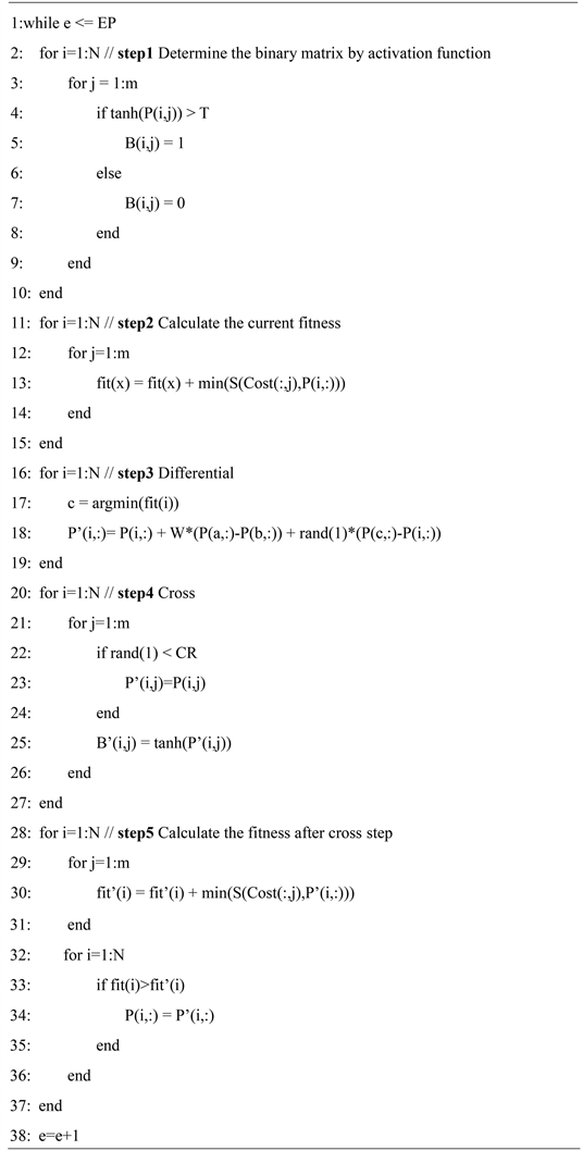
Algorithm 1. IADEA.
4. Numerical Analysis
To verify the feasibility of the IADEA and to evaluate its performance, 18 test problems from the UFL benchmark problem library are selected for solution. Then, the computational results of the basic differential evolution algorithm, IADEA and the hybrid ant colony algorithm are compared and analyzed.
4.1. Experimental Environment and Parameter Settings
The basic differential evolution algorithm and IADEA were coded on the Matlab R2017b, and all experiments are conducted on: Intel(R) Core(TM) i7-10875H CPU @2.30 GHz, 16.0 GB RAM, 64-bit Windows10.
To determine the population size N in this paper, we test the IADEA to solve the instance ga250a1 with various population size, ranging from 5 to 60. The total iterations of every population is 100 and the optimal value of this instance is 257,969.
As displayed in Table 1, the increasement in the population size bring better target value, but when the size is bigger than 20, the difference in the target value is slight compared to the difference in the elapsed time, which also increases in multiple-rate due to the larger size of population. Therefore, we decide to let the population = 20 for more efficiency.
The threshold T of the activation function determine the opening of the facility in the algorithm, if T < 0, it means more facility will be closed in the iteration, otherwise more facility will open. To applied to all instances, we let the T = 0.
The upper bound Pmax and the lower bound Pmin are related to the coefficient w in the adaptive operator and the random number in the differential step, but the upper limit of random number is 1 in the paper, so the magnitude of the Pmax and Pmin will not make a difference in the algorithm, and we set the
. Note that if
, the possibility of the opening and closing of the facility will not be the same in the algorithm, which is similar to the threshold T.
According to the discussion above and previous research, the parameters in the IADEA is set as follow: threshold T = 0, the upper bound Pmax = 30, the lower bound Pmin = −30, Wmax = 0.6, w = 0.05, Wmin = 0.3.
![]()
Table 1. The target values obtained by using different population size N.
The hybrid ant colony algorithm in the literature [12] was conducted on: Intel(R) Core(TM) i7-3770 CPU @3.4 GHz, 3.41 GB RAM, Windows 7, and data processing was done by Matlab2010.
4.2. Computational Results
Table 2 shows the computational results of the basic differential evolution algorithm and IADEA for 18 instances from the UFL benchmark problem library in the same experimental setting, where the number of facilities m and the number of customers n are equal in all problems. The target value refers to the optimal value in the population after 100 iterations and the optimal value indicate the known optimal value. The Gap value is the difference between the target value and the known optimal value, which is given by:
![]()
Table 2. The comparison of computational results between basic DE and IADEA.
![]()
Table 3. The computational result of hybrid ant colony algorithm.
As can be seen from Table 2, the introduction of the adaptive factor does not make a significant difference in the elapsed time between basic differential algorithm and IADEA for the same number of iterations, but the solution results of the IADEA are substantially better than those of the basic differential evolution algorithm. Mainly because the adaptive factor alleviates the defect that the basic differential evolution algorithm tend to fall into local optimal in the optimization process. Moreover, 12 Gap values of all 18 instances are below 8%, which proves that the adaptive differential algorithm is able to effectively find a satisfactory solution to the problem.
A comparison between Table 2 and Table 3 shows that IADEA outperforms the hybrid ant colony algorithm in all 18 instances except the ga250a1 and gs250a1 with similar or lower elapsed time.
5. Conclusions
This paper improves the basic differential evolution algorithm and proposes a differential evolution algorithm for the UFL problem based on the characteristics of the UFL problem. The proposed approach for solving UFL problem is based on the DE algorithm. To map the variable in the DE algorithm into binary one, we use the activation function to transform variables. Meanwhile, to improve the efficiency of the algorithm, we introduce the adaptive operator to alleviate the issue of being stuck in a local optimum.
It is demonstrated that the IADEA is feasible for solving the UFL problem and significantly improves the optimization efficiency of the basic differential evolution algorithm. At the same time, the IADEA can obtain better target values in similar or shorter time compared with the hybrid ant colony algorithm.
Therefore, this paper provides a new solution to the UFL problem and extends the application of the differential evolution algorithm. Further research is required to improve the convergence speed and operational efficiency of this algorithm.
NOTES
*Corresponding author.