Fast High Order Algorithm for Three-Dimensional Helmholtz Equation Involving Impedance Boundary Condition with Large Wave Numbers

Chengjie Tong, Xianqi Fang, Meiling Zhao

School of Mathematics and Physics, North China Electric Power University, Baoding, China.

DOI: 10.4236/ajcm.2023.132011                

Abstract

Acoustic fields with impedance boundary conditions have high engineering applications, such as noise control and evaluation of sound insulation materials, and can be approximated by three-dimensional Helmholtz boundary value problems. Finite difference method is widely applied to solving these problems due to its ease of use. However, when the wave number is large, the pollution effects are still a major difficulty in obtaining accurate numerical solutions. We develop a fast algorithm for solving three-dimensional Helmholtz boundary problems with large wave numbers. The boundary of computational domain is discrete based on high-order compact difference scheme. Using the properties of the tensor product and the discrete Fourier sine transform method, the original problem is solved by splitting it into independent small tridiagonal subsystems. Numerical examples with impedance boundary conditions are used to verify the feasibility and accuracy of the proposed algorithm. Results demonstrate that the algorithm has a fourth- order convergence in  and -norms, and costs less CPU calculation time and random access memory.

Keywords

Impedance Boundary Condition, Helmholtz Equation, Compact Finite Difference, Fourier Sine Transform, Large Wave Numbers

1. Introduction

Acoustics is a branch of physics with high application value in military [1] [2] , medical [3] [4] [5] and other fields [6] [7] [8] . After S. A. Schelkunoff introduced the concept of impedance into electromagnetic fields [9] , the concept of impedance was gradually incorporated into various research fields. The impedance boundary condition (IBC), also called Shchukin-Leontovich condition, was first derived by A. N. Shchukin in 1940 [10] . In the same period, a detailed derivation of IBC was published by M. A. Leontovich [11] [12] . Inspired by Leontovich, Ya. L. Alpert first applied IBCs to the practical problems of electromagnetic waves propagation [13] . Since then, an increasing number of problems involving IBCs have been studied. In practical acoustic problems, such as indoor sound insulation [14] [15] [16] and noise control [17] [18] , sound-absorbing materials are fairly common and are usually considered as IBCs [19] . Therefore, impedance boundary conditions are of significance in acoustic engineering analysis and calculation.

To solve the acoustic field with impedance boundary conditions, the finite element method (FEM) and the boundary element method (BEM) have attracted much attention. For the problems of two-dimensional acoustic pressure field with large uncertain-but-bounded parameters, a modified sub-interval perturbation FEM is presented to reduce the dependency phenomenon of parameters, and has a remarkable performance in two-dimensional tube and cavity of a vehicle [20] . In [21] , Xia and Yu proposed an interval perturbation FEM and a modified interval perturbation FEM.

Calculation of three-dimensional acoustic field is more challenging in both accuracy and efficiency. Additionally, when the frequency of acoustic waves is high, these standard mesh methods often exhibit the so-called “pollution effect” [22] . It is also a computational challenge to solve the problems within acceptable error for standard mesh methods. In this case, various numerical methods are presented to reduce the pollution effect [23] [24] [25] . However, these FEM-related methods still need a large amount of computing time and memory to solve the three-dimensional large wavenumber problem. Moreover, the pollution effect caused by the increase of wavenumber has not been completely solved.

For finite difference method [26] [27] , high-order schemes can be obtained by using the topological advantages of structured grids, which reduces the workload of computing area processing. Moreover, in [28] [29] , it is a remarkable fact that fast Fourier transform technique is introduced to solve linear difference systems, which substantially reduce both the time consumption and the memory consumption in calculation process. Nevertheless, there is still a drawback that the algorithms in [28] [29] can only solve Dirichlet boundary value problems or the boundary value problems with Neumann and Dirichlet boundary conditions. This drawback limits the practical application of the algorithms.

In this paper, a high order fast algorithm is proposed to solve the three-dimensional Helmholtz boundary value problems involving impedance boundary condition. By 19-point finite difference stencil, we discretize the Helmholtz equation and the impedance boundary condition to obtain the fourth-order compact difference scheme. Meanwhile, discrete fast Fourier sine transform is used to simplify the linear systems to be solved. Furthermore, we apply the parallel techniques in programming to accelerate the calculation process.

The outline of this paper is as follows. The model studied in this paper is introduced in Section 2. Fourth-order compact schemes of three-dimensional Helmholtz equation and discretization of impedance boundary condition are derived in Section 3 and Section 4, respectively. In Section 5, a fast algorithm with forth-order convergence is developed based on fast Fourier sine transform and Gaussian elimination. In Section 6, we present three numerical experiments to illustrate the performance of the algorithm. Several conclusions are finally drawn in Section 7.

2. Model Problem

Assuming the propagation of small amplitude acoustic wave is in a homogeneous ideal fluid, the wave equation in three-dimensional space is described as

$\frac{1}{c^2}\frac{{\partial }^{2}p}{\partial t^2}=\left(\frac{{\partial }^2}{\partial x^2}+\frac{{\partial }^2}{\partial y^2}+\frac{{\partial }^2}{\partial z^2}\right)p,$ (1)

where p denotes the pressure of acoustic wave and c is the velocity of sound. The function of pressure p is given by

$p\left(x\mathrm{,}y\mathrm{,}z\mathrm{,}t\right)=\Re \mathfrak{e}\left(\psi \left(x\mathrm{,}y\mathrm{,}z\right){\text{e}}^{-\text{i}\omega t}\right)\mathrm{,}$ (2)

where $\Re \mathfrak{e}$ denotes the real parts and $\psi$ represents the complex time harmonic pressure. $\omega$ is the angular frequency (rad/s) and $\text{i}=\sqrt{-1}$ is imaginary unit. Separating the variables of Equation (1) to obtain the time-independent form, the spatial distribution of acoustic pressure satisfies the Helmholtz equation $\Delta \psi +{\kappa }^2\psi =0$ with appropriate boundary conditions, where $\Delta$ denotes the Laplace operator and $\kappa$ is the acoustic wave number given by $\kappa =\omega /c$ .

Without loss of generality, the problem studied in this paper is a Helmholtz boundary value problem in a three-dimensional continuous convex doman $\mathcal{D}\subset {ℝ}^3$ . The boundary conditions on $\partial D$ are mixed, involving a general impedance boundary condition on ${\Gamma }_I$ and a Dirichlet boundary on ${\Gamma }_D=\partial D\backslash {\Gamma }_I$ . The model problem can be described as follows

$\Delta \psi +{\kappa }^2\psi =f\mathrm{,}\text{in}\mathcal{D}\mathrm{,}$ (3a)

$\psi =b\mathrm{,}\text{on}{\Gamma }_D\mathrm{,}$ (3b)

$n\cdot \nabla \psi +\text{i}\kappa \beta \psi =g\mathrm{,}\text{on}{\Gamma }_I\mathrm{,}$ (3c)

where $f\left(x\mathrm{,}y\mathrm{,}z\right)$ , $b\left(x\mathrm{,}y\mathrm{,}z\right)$ and $g\left(x\mathrm{,}y\right)$ are known functions. $n$ is the unit outward normal to ${\Gamma }_I$ , and $\nabla$ represents the gradient operator. $\beta$ denotes the relative surface admittance coefficient of sturctural damping. Generally, $\beta$ is a function of frequency and position.

If $\psi \equiv 0$ in Equation (3b), the boundary condition on ${\Gamma }_D$ is called sound soft boundary. In Equation (3c), function g on the right side represents the flow across ${\Gamma }_I$ . Different from radiation problems, the sound source term g is set to zero in acoustic scattering problems. Additionally, the Neumann boundary condition is obtained if the value of $\beta$ is set to 0. Furthermore, the boundary ${\Gamma }_I$ is sound hard or acoustically rigid in the case of $g=0$ . If the valve of f, b and g are identically zero, and $\beta$ is set to non-zero, this model is degenerate into the steady-state acoustic pressure field oscillations involving an impedance boundary condition as follows.

3. Discretization of There-Dimensional Helmholtz Equation

We assume that the domain of propagation $\mathcal{D}$ is cubic, and ${\Gamma }_I$ is the upper surface. The domain $\mathcal{D}=\left[x_{\text{min}}\mathrm{,}{x}_{\text{max}}\right]\times \left[y_{\text{min}}\mathrm{,}{y}_{\text{max}}\right]\times \left[z_{\text{min}}\mathrm{,}{z}_{\text{max}}\right]$ is divided into a uniform partition in steps $h_x=\frac{x_{\text{max}}-x_{\text{min}}}{M+1}$ , $h_y=\frac{y_{\text{max}}-y_{\text{min}}}{N+1}$ and $h_z=\frac{z_{\text{max}}-z_{\text{min}}}{K+1}$ along the axes. ${\left\{x_i,y_j,z_k\right\}}_{i,j,k=0}^{M+1,N+1,K+1}$ denotes the set of grids, where M, N and K are the numbers of internal grids in each directions. Figure 1 illustrates the geometric structure of the model problem (3) and the 19-points finite difference stencil. In Figure 1, the central point is marked red. Blue and black represent all face-centered and all edge-centered points, respectively.

Without losing generality, equal step size $h=h_x=h_y=h_z$ is taken on each axes. Approximated by fourth-order Taylor series expansion at $\left(x_i\mathrm{,}{y}_j\mathrm{,}{z}_k\right)$ , we can derive

$\begin{array}{l}{\psi }_{xx}\left(x_i,y_j,z_k\right)={\left(1+\frac{h^2}{12}{\delta }_x^2\right)}^{-1}{\delta }_x^2{\psi }_{i,j,k}+\mathcal{O}\left(h^4\right),\\ {\delta }_x^2{\psi }_{i,j,k}=\frac{1}{h^2}\left({\psi }_{i+1,j,k}-2{\psi }_{i,j,k}+{\psi }_{i-1,j,k}\right),\end{array}$ (4)

where ${\psi }_{xx}$ is the second-order partial derivative of $\psi$ with respect to x, and ${\delta }_x^2$ denotes the standard second-order central difference operator in the x-direction. ${\psi }_{i\mathrm{,}j\mathrm{,}k}=\psi \left(x_i\mathrm{,}{y}_j\mathrm{,}{z}_k\right)$ is the solution of $\psi$ at Let $\left(x_i\mathrm{,}{y}_j\mathrm{,}{z}_k\right)$ . The approximation of ${\psi }_{yy}$ and ${\psi }_{zz}$ can be derived in the same way, i.e.

Figure 1. The geometric structure of the model problem and the 19-points finite difference stencil.

$\begin{array}{l}{\psi }_{yy}\left(x_i\mathrm{,}{y}_j\mathrm{,}{z}_k\right)={\left(1+\frac{h^2}{12}{\delta }_y^2\right)}^{-1}{\delta }_y^2{\psi }_{i\mathrm{,}j\mathrm{,}k}+\mathcal{O}\left(h^4\right)\mathrm{,}\\ {\psi }_{zz}\left(x_i\mathrm{,}{y}_j\mathrm{,}{z}_k\right)={\left(1+\frac{h^2}{12}{\delta }_z^2\right)}^{-1}{\delta }_z^2{\psi }_{i\mathrm{,}j\mathrm{,}k}+\mathcal{O}\left(h^4\right)\mathrm{,}\end{array}$ (5)

where

$\begin{array}{l}{\delta }_y^2{\psi }_{i\mathrm{,}j\mathrm{,}k}=\frac{1}{h^2}\left({\psi }_{i\mathrm{,}j+\mathrm{1,}k}-2{\psi }_{i\mathrm{,}j\mathrm{,}k}+{\psi }_{i\mathrm{,}j-\mathrm{1,}k}\right)\mathrm{,}\\ {\delta }_z^2{\psi }_{i\mathrm{,}j\mathrm{,}k}=\frac{1}{h^2}\left({\psi }_{i\mathrm{,}j\mathrm{,}k+1}-2{\psi }_{i\mathrm{,}j\mathrm{,}k}+{\psi }_{i\mathrm{,}j\mathrm{,}k-1}\right)\mathrm{.}\end{array}$ (6)

Combining Equations (3a), (4), (5) and (6), the compact fourth-order difference scheme for Helmholtz equation is obtained as follows

$T_0{\psi }_{i\mathrm{,}j\mathrm{,}k}=\left(1+\frac{h^2}{12}\Delta \right)f_{i\mathrm{,}j\mathrm{,}k}+\mathcal{O}\left(h^4\right)\mathrm{,}$ (7)

where

$T_0=\left(1+\frac{{\kappa }^2{h}^2}{12}\right)\left({\delta }_x^2+{\delta }_y^2+{\delta }_z^2\right)+\frac{h^2}{6}\left({\delta }_x^2{\delta }_y^2+{\delta }_y^2{\delta }_z^2+{\delta }_x^2{\delta }_z^2\right)+{\kappa }^2\mathrm{.}$

The truncation error of Equation (7) is

$\begin{array}{l}E=\left(\frac{{\kappa }^2}{144}\left({\psi }_{x^4}+{\psi }_{y^4}\right)+\frac{1}{360}\left({\psi }_{x^6}+{\psi }_{y^6}\right)+\frac{1}{72}\left({\psi }_{x^4{y}^2}+{\psi }_{x^2{y}^4}\right)\right)h^4\\ -\frac{h^4}{144}\left(f_{x^4}+f_{y^4}\right)\mathrm{.}\end{array}$ (8)

Note that $\Delta f_{i\mathrm{,}j\mathrm{,}k}$ should be substituted by $\left({\delta }_x^2+{\delta }_y^2+{\delta }_z^2\right)f_{i\mathrm{,}j\mathrm{,}k}$ , if f is not second-order differentiable. Multiplying $h^2$ on the both sides and substituting ${\delta }_z^2$ in Equation (6), Equation (7) can be rewritten as

$\begin{array}{l}{T}_1\left({\psi }_{i,j,k-1}+{\psi }_{i,j,k+1}\right)+T_2{\psi }_{i,j,k}=\left(h^2+\frac{h^4}{12}\Delta \right)f_{i,j,k},\\ i=1,2,\cdots ,M;j=1,2,\cdots ,N;k=1,2,\cdots ,K.\end{array}$ (9)

where

$\begin{array}{l}{T}_1=1+\frac{{\kappa }^2{h}^2}{12}+\frac{h^2}{6}\left({\delta }_x^2+{\delta }_y^2\right),\\ T_2=\left(\frac{{\kappa }^2{h}^4}{12}+\frac{2h^2}{3}\right)\left({\delta }_x^2+{\delta }_y^2\right)+\frac{h^4}{6}\left({\delta }_x^2{\delta }_y^2\right)+\frac{5{\kappa }^2{h}^2}{6}-2.\end{array}$ (10)

For convenience, we introduce the tridiagonal Toeplitz matrix $D=\frac{1}{h^2}\text{tridiag}\left(\mathrm{1,}-\mathrm{2,1}\right)$ . Thus, Equation (7) can be written in the matrix form as

$\begin{array}{l}\left(1+\frac{{\kappa }^2{h}^2}{12}\right)\left(D_M\otimes I_N\otimes I_K+I_M\otimes D_N\otimes I_K+I_M\otimes I_N\otimes D_K\right)\Psi \\ +\frac{h^2}{6}\left(D_M\otimes D_N\otimes I_K+I_M\otimes D_N\otimes D_K+D_M\otimes I_N\otimes D_K\right)\Psi +{\kappa }^2\Psi +{\Psi }_B\\ =\frac{h^2}{12}\left(D_M\otimes I_N\otimes I_K+I_M\otimes D_N\otimes I_K+I_M\otimes I_N\otimes D_K\right)F+F+F_B\mathrm{.}\end{array}$ (11)

Here the symbol $\otimes$ denotes the Kronecker product. The sizes of $D_M$ , $D_N$ and $D_K$ are $M\times M$ , $N\times N$ , $K\times K$ , respectively. $I_M$ , $I_N$ , $I_K$ are identity matrices, and

$\begin{array}{l}\Psi ={\left({\psi }_{\mathrm{1,1,1}}\mathrm{,}\cdots \mathrm{,}{\psi }_{\mathrm{1,1,}K}\mathrm{,}{\psi }_{\mathrm{1,2,1}}\mathrm{,}\cdots \mathrm{,}{\psi }_{\mathrm{1,2,}K}\mathrm{,}\cdots \mathrm{,}{\psi }_{\mathrm{1,}N\mathrm{,}K}\mathrm{,}\cdots \mathrm{,}{\psi }_{M\mathrm{,}N\mathrm{,}K}\right)}^{\text{T}}\mathrm{,}\\ F={\left(f_{\mathrm{1,1,1}}\mathrm{,}\cdots \mathrm{,}{f}_{\mathrm{1,1,}K}\mathrm{,}{f}_{\mathrm{1,2,1}}\mathrm{,}\cdots \mathrm{,}{f}_{\mathrm{1,2,}K}\mathrm{,}\cdots \mathrm{,}{f}_{\mathrm{1,}N\mathrm{,}K}\mathrm{,}\cdots \mathrm{,}{f}_{M\mathrm{,}N\mathrm{,}K}\right)}^{\text{T}}\mathrm{.}\end{array}$

${\Psi }_B$ and $F_B$ are the boundary parts not included in Ψ and F, respectively. In details, we can derive

$\begin{array}{c}{F}_B=\left(1+\frac{{\kappa }^2{h}^2}{12}\right)\left(a_{M1}\otimes I_N\otimes I_K\right)F_{\mathrm{0,\; <mo>\; :\; </mo>,\; <mo>\; :\; </mo>}}+\left(1+\frac{{\kappa }^2{h}^2}{12}\right)\left(a_{M2}\otimes I_N\otimes I_K\right)F_{\mathrm{<mo>\; :\; </mo>,\; <mo>\; :\; </mo>,}M+1}\\ +\left(1+\frac{{\kappa }^2{h}^2}{12}\right)\left(I_M\otimes a_{N1}\otimes I_K\right)F_{\mathrm{<mo>\; :\; </mo>,0,\; <mo>\; :\; </mo>}}+\left(1+\frac{{\kappa }^2{h}^2}{12}\right)\left(I_M\otimes a_{N2}\otimes I_K\right)F_{\mathrm{<mo>\; :\; </mo>,}N+\mathrm{1,\; <mo>\; :\; </mo>}}\\ +\left(1+\frac{{\kappa }^2{h}^2}{12}\right)\left(I_M\otimes I_N\otimes a_{K1}\right)F_{\mathrm{<mo>\; :\; </mo>,\; <mo>\; :\; </mo>,0}}+\left(1+\frac{{\kappa }^2{h}^2}{12}\right)\left(I_M\otimes I_N\otimes a_{K2}\right)F_{\mathrm{<mo>\; :\; </mo>,\; <mo>\; :\; </mo>,}K+1}\mathrm{,}\end{array}$ (12)

where

$\begin{array}{l}{a}_{M1}=\frac{1}{h^2}{\left(\mathrm{1,0,}\cdots \mathrm{,0}\right)}_M^{\text{T}}\mathrm{,}{a}_{N1}=\frac{1}{h^2}{\left(\mathrm{1,0,}\cdots \mathrm{,0}\right)}_N^{\text{T}}\mathrm{,}\\ a_{K1}=\frac{1}{h^2}{\left(\mathrm{1,0,}\cdots \mathrm{,0}\right)}_K^{\text{T}}\mathrm{,}{a}_{M2}=\frac{1}{h^2}{\left(\mathrm{0,0,}\cdots \mathrm{,1}\right)}_M^{\text{T}}\mathrm{,}\\ a_{N2}=\frac{1}{h^2}{\left(\mathrm{0,0,}\cdots \mathrm{,1}\right)}_N^{\text{T}}\mathrm{,}{a}_{K2}=\frac{1}{h^2}{\left(\mathrm{0,0,}\cdots \mathrm{,1}\right)}_K^{\text{T}}\mathrm{.}\end{array}$ (13)

For ${\Psi }_B$ , it is divided into edge part ${\Psi }_{BE}$ and surface part ${\Psi }_{BS}$ as

$\begin{array}{c}{\Psi }_{BE}=\frac{h^2}{6}\left(a_{M1}\otimes I_N\otimes a_{K1}\right){\Psi }_{\mathrm{0,\; <mo>\; :\; </mo>,0}}+\frac{h^2}{6}\left(a_{M2}\otimes I_N\otimes a_{K1}\right){\Psi }_{M+\mathrm{1,\; <mo>\; :\; </mo>,0}}\\ +\frac{h^2}{6}\left(I_M\otimes a_{N1}\otimes a_{K1}\right){\Psi }_{\mathrm{<mo>\; :\; </mo>,0,0}}+\frac{h^2}{6}\left(I_M\otimes a_{N2}\otimes a_{K1}\right){\Psi }_{\mathrm{<mo>\; :\; </mo>,}N+\mathrm{1,0}}\\ +\frac{h^2}{6}\left(a_{M1}\otimes a_{N1}\otimes I_K\right){\Psi }_{\mathrm{0,0,\; <mo>\; :\; </mo>}}+\frac{h^2}{6}\left(a_{M1}\otimes a_{N2}\otimes I_K\right){\Psi }_{\mathrm{0,}K+\mathrm{1,\; <mo>\; :\; </mo>}}\\ +\frac{h^2}{6}\left(a_{M2}\otimes a_{N1}\otimes I_K\right){\Psi }_{M+\mathrm{1,0,\; <mo>\; :\; </mo>}}+\frac{h^2}{6}\left(a_{M2}\otimes a_{N2}\otimes I_K\right){\Psi }_{M+\mathrm{1,}K+\mathrm{1,\; <mo>\; :\; </mo>}}\\ +\frac{h^2}{6}\left(a_{M1}\otimes I_N\otimes a_{K2}\right){\Psi }_{\mathrm{0,\; <mo>\; :\; </mo>,}K+1}+\frac{h^2}{6}\left(a_{M2}\otimes I_N\otimes a_{K2}\right){\Psi }_{M+\mathrm{1,\; <mo>\; :\; </mo>,}K+1}\\ +\frac{h^2}{6}\left(I_M\otimes a_{N1}\otimes a_{K2}\right){\Psi }_{\mathrm{<mo>\; :\; </mo>,0,}K+1}+\frac{h^2}{6}\left(I_M\otimes a_{N2}\otimes a_{K2}\right){\Psi }_{\mathrm{<mo>\; :\; </mo>,}N+\mathrm{1,}K+1}\mathrm{,}\end{array}$ (14)

and

$\begin{array}{c}{\Psi }_{BS}={\Psi }_{BI}+\frac{h^2}{6}\left(a_{M1}\otimes D_N\otimes I_K+a_{M1}\otimes I_N\otimes D_K\right){\Psi }_{\mathrm{0,\; <mo>\; :\; </mo>,\; <mo>\; :\; </mo>}}\\ +\frac{h^2}{6}\left(a_{M2}\otimes D_N\otimes I_K+a_{M2}\otimes I_N\otimes D_K\right){\Psi }_{M+\mathrm{1,\; <mo>\; :\; </mo>,\; <mo>\; :\; </mo>}}\\ +\frac{h^2}{6}\left(D_M\otimes a_{N1}\otimes I_K+I_M\otimes a_{N1}\otimes D_K\right){\Psi }_{\mathrm{<mo>\; :\; </mo>,0,\; <mo>\; :\; </mo>}}\\ +\frac{h^2}{6}\left(D_M\otimes a_{N2}\otimes I_K+I_M\otimes a_{N2}\otimes D_K\right){\Psi }_{\mathrm{<mo>\; :\; </mo>,}N+\mathrm{1,\; <mo>\; :\; </mo>}}\\ +\frac{h^2}{6}\left(D_M\otimes I_N\otimes a_{K1}+I_M\otimes D_N\otimes a_{K1}\right){\Psi }_{\mathrm{<mo>\; :\; </mo>,\; <mo>\; :\; </mo>,0}}\end{array}$

$\begin{array}{c}+\left(1+\frac{{\kappa }^2{h}^2}{12}\right)\left(a_{M1}\otimes I_N\otimes I_K\right){\Psi }_{\mathrm{0,\; <mo>\; :\; </mo>,\; <mo>\; :\; </mo>}}+\left(1+\frac{{\kappa }^2{h}^2}{12}\right)\left(a_{M2}\otimes I_N\otimes I_K\right){\Psi }_{M+\mathrm{1,\; <mo>\; :\; </mo>,\; <mo>\; :\; </mo>}}\\ +\left(1+\frac{{\kappa }^2{h}^2}{12}\right)\left(I_M\otimes a_{N1}\otimes I_K\right){\Psi }_{\mathrm{<mo>\; :\; </mo>,0,\; <mo>\; :\; </mo>}}+\left(1+\frac{{\kappa }^2{h}^2}{12}\right)\left(I_M\otimes a_{N2}\otimes I_K\right){\Psi }_{\mathrm{<mo>\; :\; </mo>,}N+\mathrm{1,\; <mo>\; :\; </mo>}}\\ +\left(1+\frac{{\kappa }^2{h}^2}{12}\right)\left(I_M\otimes I_N\otimes a_{K1}\right){\Psi }_{\mathrm{<mo>\; :\; </mo>,\; <mo>\; :\; </mo>,0}}\mathrm{,}\end{array}$ (15)

where ${\Psi }_{BI}$ is discrete value of solution on the impedance boundary ${\Gamma }_I$ . Since the function $b\left(x\mathrm{,}y\mathrm{,}z\right)$ is known, the solution of $\psi$ on ${\Gamma }_D$ can be replaced. Moreover, we can rewrite Equation (11) as follows

$\begin{array}{c}\left(1+\frac{{\kappa }^2{h}^2}{12}\right)\left(D_M\otimes I_N\otimes I_K+I_M\otimes D_N\otimes I_K+I_M\otimes I_N\otimes D_K\right)\Psi \\ +\frac{h^2}{6}\left(D_M\otimes D_N\otimes I_K+I_M\otimes D_N\otimes D_K+D_M\otimes I_N\otimes D_K\right)\Psi +{\kappa }^2\Psi \\ +\left(\left(1+\frac{{\kappa }^2{h}^2}{12}\right)I_M\otimes I_N\otimes a_{K2}+\frac{h^2}{6}\left(D_M\otimes I_N+I_M\otimes D_N\right)\otimes a_{K2}\right){\Psi }_{\mathrm{<mo>\; :\; </mo>,\; <mo>\; :\; </mo>,}K+1}\\ =\frac{h^2}{12}\left(D_M\otimes I_N\otimes I_K+I_M\otimes D_N\otimes I_K+I_M\otimes I_N\otimes D_K\right)F+F+F_B-{\Psi }_{BD}\mathrm{,}\end{array}$ (16)

where ${\Psi }_{BD}={\Psi }_B-{\Psi }_I$ .

4. Discretization of Impedance Boundary Condition

To obtain the fourth-order difference approximation with Taylor series expansion, we discrete the impedance boundary condition in Equation (3c). The left term can be written as

$\begin{array}{l}{\left(n\cdot \nabla \psi +\text{i}\kappa \beta \psi \right)}_{i\mathrm{,}j\mathrm{,}K}\\ =\frac{{\psi }_{i\mathrm{,}j\mathrm{,}K+2}-{\psi }_{i\mathrm{,}j\mathrm{,}K}}{2h}-\frac{h^2}{6}{\left({\psi }_{zzz}\right)}_{i\mathrm{,}j\mathrm{,}K+1}+\text{i}\beta \kappa {\psi }_{i\mathrm{,}j\mathrm{,}K+1}\\ +\mathcal{O}\left(h^4\right)\mathrm{,}i=\mathrm{1,2,}\cdots \mathrm{,}M;j=\mathrm{1,2,}\cdots \mathrm{,}N\mathrm{,}\end{array}$ (17)

where ${\psi }_{i\mathrm{,}j\mathrm{,}K+2}$ is the ghost points outside the model domain $\mathcal{D}$ . Taking the partial derivatives of z on both sides of Helmholtz Equation (Equation (3a)), we can obtain the third-order partial derivative as follows

${\psi }_{zzz}=-{\psi }_{xxz}-{\psi }_{yyz}-{\kappa }^2{\psi }_z+f_z.$ (18)

Further, Equation (18) can be approximated as

$\begin{array}{l}{\psi }_{zzz}=-\left({\delta }_x^2+{\delta }_y^2+{\kappa }^2\right)\frac{{\psi }_{i,j,K+2}-{\psi }_{i,j,K}}{2h}+f_z.\hfill \end{array}$ (19)

After substitution of (17) and (19) into (3c), the expression is given by

$\begin{array}{l}\left(1+\frac{h^2}{6}\left({\delta }_x^2+{\delta }_y^2+{\kappa }^2\right)\right)\frac{{\psi }_{i\mathrm{,}j\mathrm{,}K+2}-{\psi }_{i\mathrm{,}j\mathrm{,}K}}{2h}+\text{i}\kappa \beta {\psi }_{i\mathrm{,}j\mathrm{,}K+1}\\ =g_{i\mathrm{,}j}+\frac{h^2}{6}{\left(f_z\right)}_{i\mathrm{,}j\mathrm{,}K+1}+\mathcal{O}\left(h^4\right)\mathrm{.}\end{array}$ (20)

Similarly, the matrix form of Equation (20) is obtained as follows

$\begin{array}{l}\left(\left(1+\frac{{\kappa }^2{h}^2}{6}\right)I_{MN}+\frac{h^2}{6}\left(D_M\otimes I_N+I_M\otimes D_N\right)\right){\Psi }_{\mathrm{<mo>\; :\; </mo>,\; <mo>\; :\; </mo>,}K+2}+\text{i}2h\kappa \beta {\Psi }_{\mathrm{<mo>\; :\; </mo>,\; <mo>\; :\; </mo>,}K+1}\\ -\left(\left(1+\frac{{\kappa }^2{h}^2}{6}\right)I_{MN}+\frac{h^2}{6}\left(D_M\otimes I_N+I_M\otimes D_N\right)\right){\Psi }_{\mathrm{<mo>\; :\; </mo>,\; <mo>\; :\; </mo>,}K}\\ =2hg+\frac{h^3}{3}{f}_z-B\mathrm{,}\end{array}$ (21)

where

$\begin{array}{l}g={\left(g_{\mathrm{1,1}}\mathrm{,}{g}_{\mathrm{1,2}}\mathrm{,}\cdots \mathrm{,}{g}_{\mathrm{1,}N}\mathrm{,}{g}_{\mathrm{2,1}}\mathrm{,}\cdots \mathrm{,}{g}_{\mathrm{2,}N}\mathrm{,}\cdots \mathrm{,}{g}_{M\mathrm{,}N}\right)}^{\text{T}}\mathrm{,}\\ f_z={\left({\left(f_z\right)}_{\mathrm{1,1}}\mathrm{,}{\left(f_z\right)}_{\mathrm{1,2}}\mathrm{,}\cdots \mathrm{,}{\left(f_z\right)}_{\mathrm{1,}N}\mathrm{,}{\left(f_z\right)}_{\mathrm{2,1}}\mathrm{,}\cdots \mathrm{,}{\left(f_z\right)}_{\mathrm{2,}N}\mathrm{,}\cdots \mathrm{,}{\left(f_z\right)}_{M\mathrm{,}N}\right)}^{\text{T}}\mathrm{,}\\ B=\frac{h^2}{6}{\left(b_{\mathrm{0,1,}K}\mathrm{,}{b}_{\mathrm{0,2,}K}\mathrm{,}\cdots \mathrm{,}{b}_{\mathrm{0,}N\mathrm{,}K}\mathrm{,0,}\cdots \mathrm{,0,}{b}_{M+\mathrm{1,1,}K}\mathrm{,}{b}_{M+\mathrm{1,2,}K}\mathrm{,}\cdots \mathrm{,}{b}_{M+\mathrm{1,}N\mathrm{,}K}\right)}^{\text{T}}\\ +\frac{h^2}{6}(b_{\mathrm{1,0,}K}\mathrm{,0,}\cdots \mathrm{,0,}{b}_{\mathrm{1,}N+\mathrm{1,}K}\mathrm{,}{b}_{\mathrm{2,0,}K}\mathrm{,0,}\cdots \mathrm{,0,}{b}_{\mathrm{2,}N+\mathrm{1,}K}\mathrm{,}\cdots \mathrm{,}{b}_{M\mathrm{,0,}K}\mathrm{,}\\ {\mathrm{0,}\cdots \mathrm{,0,}{b}_{M\mathrm{,}N+\mathrm{1,}K})}^{\text{T}}\mathrm{.}\end{array}$

We denote $L_1=\left(1+\frac{{\kappa }^2{h}^2}{6}\right)I_{MN}+\frac{h^2}{6}\left(D_M\otimes I_N+I_M\otimes D_N\right)$ , and $L_1$ is invertible if the h is small enough. Thus, we have

${\Psi }_{\mathrm{<mo>\; :\; </mo>,\; <mo>\; :\; </mo>,}K+2}={\Psi }_{\mathrm{<mo>\; :\; </mo>,\; <mo>\; :\; </mo>,}K}+L_1^{-1}\left(2hg+\frac{h^3}{3}{f}_z-B-\text{i}2h\kappa \beta {\Psi }_{\mathrm{<mo>\; :\; </mo>,\; <mo>\; :\; </mo>,}K+1}\right)\mathrm{.}$ (22)

Replacing k in Equation (9) with $K+1$ , we have

$T_1\left({\psi }_{i\mathrm{,}j\mathrm{,}K}+{\psi }_{i\mathrm{,}j\mathrm{,}K+2}\right)+T_2{\psi }_{i\mathrm{,}j\mathrm{,}K+1}=\left(h^2+\frac{h^4}{12}\Delta \right)f_{i\mathrm{,}j\mathrm{,}K+1}\mathrm{,}$ (23)

and the matrix form as follows

$\begin{array}{l}(\left(\frac{{\kappa }^2{h}^4}{12}+\frac{h^2}{3}\right)\left(D_M\otimes I_N+I_M\otimes D_N\right)+\frac{h^4}{6}{D}_M\otimes D_N\\ +\left(\frac{5{\kappa }^2{h}^2}{6}-2\right)I_{MN}){\Psi }_{\mathrm{<mo>\; :\; </mo>,\; <mo>\; :\; </mo>,}K+1}\\ +\left(\left(1+\frac{{\kappa }^2{h}^2}{12}\right)I_{MN}+\frac{h^2}{6}\left(D_M\otimes I_N+I_M\otimes D_N\right)\right){\Psi }_{\mathrm{<mo>\; :\; </mo>,\; <mo>\; :\; </mo>,}K+2}\\ +\left(\left(1+\frac{{\kappa }^2{h}^2}{12}\right)I_{MN}+\frac{h^2}{6}\left(D_M\otimes I_N+I_M\otimes D_N\right)\right){\Psi }_{\mathrm{<mo>\; :\; </mo>,\; <mo>\; :\; </mo>,}K}\\ =h^2{F}_{\mathrm{<mo>\; :\; </mo>,\; <mo>\; :\; </mo>,}K+1}+\frac{h^4}{12}\Delta F_{\mathrm{<mo>\; :\; </mo>,\; <mo>\; :\; </mo>,}K+1}\mathrm{.}\end{array}$ (24)

Denoting $L_2=\left(1+\frac{{\kappa }^2{h}^2}{12}\right)I_{MN}+\frac{h^2}{6}\left(D_M\otimes I_N+I_M\otimes D_N\right)$ and substituting Equation (22) into Equation (24), we have

$\begin{array}{l}(\left(\frac{{\kappa }^2{h}^4}{12}+\frac{h^2}{3}\right)\left(D_M\otimes I_N+I_M\otimes D_N\right)+\frac{h^4}{6}{D}_M\otimes D_N\\ +\left(\frac{5{\kappa }^2{h}^2}{6}-2\right)I_{MN}){\Psi }_{\mathrm{<mo>\; :\; </mo>,\; <mo>\; :\; </mo>,}K+1}-\text{i}2h\kappa \beta L_2{L}_1^{-1}{\Psi }_{\mathrm{<mo>\; :\; </mo>,\; <mo>\; :\; </mo>,}K+1}\\ +2\left(\left(1+\frac{{\kappa }^2{h}^2}{12}\right)I_{MN}+\frac{h^2}{6}\left(D_M\otimes I_N+I_M\otimes D_N\right)\right){\Psi }_{\mathrm{<mo>\; :\; </mo>,\; <mo>\; :\; </mo>,}K}\\ =-2h{L}_2{L}_1^{-1}g-\frac{h^3}{3}{L}_2{L}_1^{-1}{f}_z+L_2{L}_1^{-1}B+h^2{F}_{\mathrm{<mo>\; :\; </mo>,\; <mo>\; :\; </mo>,}K+1}+\frac{h^4}{12}\Delta F_{\mathrm{<mo>\; :\; </mo>,\; <mo>\; :\; </mo>,}K+1}\mathrm{.}\end{array}$ (25)

5. Fast Algorithm Based on Discrete Fourier Sine Transform

Combining Equation (16) and (25), the linear system is obtained from the compact fourth-order difference schemes as follows

$\left(\begin{array}{cc}{A}_{11}& A_{12}\\ A_{21}& A_{22}\end{array}\right)\left(\begin{array}{c}\Psi \\ {\Psi }_{\mathrm{<mo>\; :\; </mo>,\; <mo>\; :\; </mo>,}K+1}\end{array}\right)=\left(\begin{array}{c}{F}_{\mathcal{D}}\\ F_{{\Gamma }_I}\end{array}\right)$ (26)

Here

$\begin{array}{l}{A}_{11}=\left(1+\frac{{\kappa }^2{h}^2}{12}\right)\left(D_M\otimes I_N\otimes I_K+I_M\otimes D_N\otimes I_K+I_M\otimes I_N\otimes D_K\right)\\ +\frac{h^2}{6}\left(D_M\otimes D_N\otimes I_K+I_M\otimes D_N\otimes D_K+D_M\otimes I_N\otimes D_K\right)+{\kappa }^2{I}_{MNK}\mathrm{,}\\ A_{12}=\left(1+\frac{{\kappa }^2{h}^2}{12}\right)I_M\otimes I_N\otimes a_{K2}+\frac{h^2}{6}\left(D_M\otimes I_N+I_M\otimes D_N\right)\otimes a_{K2}\mathrm{,}\\ A_{21}=2\left(\left(1+\frac{{\kappa }^2{h}^2}{12}\right)I_{MN}+\frac{h^2}{6}\left(D_M\otimes I_N+I_M\otimes D_N\right)\right)\otimes h^2{a}_{K2}^{\text{T}}\mathrm{,}\\ A_{22}=(\left(\frac{{\kappa }^2{h}^4}{12}+\frac{h^2}{3}\right)\left(D_M\otimes I_N+I_M\otimes D_N\right)+\frac{h^4}{6}{D}_M\otimes D_N\\ +\left(\frac{5{\kappa }^2{h}^2}{6}-2\right)I_{MN})-\text{i}2h\kappa \beta L_2{L}_1^{-1}{I}_{MN}\mathrm{,}\end{array}$

$\begin{array}{l}{F}_{{\Gamma }_I}=-2h{L}_2{L}_1^{-1}g-\frac{h^3}{3}{L}_2{L}_1^{-1}{f}_z+L_2{L}_1^{-1}B+h^2{F}_{\mathrm{<mo>\; :\; </mo>,\; <mo>\; :\; </mo>,}K+1}+\frac{h^4}{12}\Delta F_{\mathrm{<mo>\; :\; </mo>,\; <mo>\; :\; </mo>,}K+1}\mathrm{,}\\ F_{\mathcal{D}}=\frac{h^2}{12}\left(D_M\otimes I_N\otimes I_K+I_M\otimes D_N\otimes I_K+I_M\otimes I_N\otimes D_K\right)F\\ +F+F_B-{\Psi }_{BD}\mathrm{.}\end{array}$

To reduce the computational complexity and accelerate the speed of solving the linear system, the Fourier sine transform (FST) is applied to improve the algorithm. The discrete Fourier sine transform matrix can be expressed as

$\begin{array}{l}{\left(T_M\right)}_{i\mathrm{,}j}=\sqrt{\frac{2}{M+1}}\left(\sin \left(\frac{ij\pi }{M+1}\right)\right)\mathrm{,}\hfill \end{array}$ (27)

and $T_M$ satisfies $T_M{T}_M=I_M$ , where M represents the size of matrices. A typical discrete FST is shown as follows

$\begin{array}{l}{T}_M{D}_M{T}_M=L_M=\text{diag}\left({\lambda }_1\mathrm{,}{\lambda }_2\mathrm{,}\cdots \mathrm{,}{\lambda }_M\right)\mathrm{,}\\ {\lambda }_i=-\frac{4{\left(M+1\right)}^2}{a^2}{\sin }^2\left(\frac{i\pi }{2\left(M+1\right)}\right)\mathrm{,}\end{array}$ (28)

where $i=1,2,\cdots ,M$ , $j=1,2,\cdots ,M$ . Replacing M in Equation (28) with N, the definitions of ${\left(T_N\right)}_{i\mathrm{,}j}$ and ${\mu }_i$ can be obtained in the same way.

Multiplying $T_M\otimes T_N$ on both sides of Equation (25), the following equation can be obtained

$2{\bar{L}}_2{\bar{\Psi }}_{\mathrm{<mo>\; :\; </mo>,\; <mo>\; :\; </mo>,}K}+{\bar{A}}_{22}{\bar{\Psi }}_{\mathrm{<mo>\; :\; </mo>,\; <mo>\; :\; </mo>,}K+1}={\bar{F}}_{{\Gamma }_I}\mathrm{,}$ (29)

where

$\begin{array}{l}{\bar{A}}_{22}=(\left(\frac{{\kappa }^2{h}^4}{12}+\frac{h^2}{3}\right)\left(L_M\otimes I_N+I_M\otimes L_N\right)+\frac{h^4}{6}{L}_M\otimes L_N\\ +\left(\frac{5{\kappa }^2{h}^2}{6}-2\right)I_{MN})-\text{i}2h\kappa \beta {\bar{L}}_2{\bar{L}}_1^{-1}{I}_{MN}\mathrm{,}\\ {\bar{L}}_1=\left(1+\frac{{\kappa }^2{h}^2}{6}\right)I_{MN}+\frac{h^2}{6}\left(L_M\otimes I_N+I_M\otimes L_N\right)\mathrm{,}\\ {\bar{L}}_2=\left(1+\frac{{\kappa }^2{h}^2}{12}\right)I_{MN}+\frac{h^2}{6}\left(L_M\otimes I_N+I_M\otimes L_N\right)\mathrm{,}\end{array}$

$\begin{array}{l}{\bar{F}}_{{\Gamma }_I}=-2h{\bar{L}}_2{\bar{L}}_1^{-1}\bar{g}-\frac{h^3}{3}{\bar{L}}_2{\bar{L}}_1^{-1}{\bar{f}}_z+{\bar{L}}_2{\bar{L}}_1^{-1}\bar{B}+h^2{\bar{F}}_{\mathrm{<mo>\; :\; </mo>,\; <mo>\; :\; </mo>,}K+1}+\frac{h^4}{12}\Delta {\bar{F}}_{\mathrm{<mo>\; :\; </mo>,\; <mo>\; :\; </mo>,}K+1}\mathrm{,}\\ \bar{g}=\left(T_M\otimes T_N\right)g\mathrm{,}{\bar{f}}_z=\left(T_M\otimes T_N\right)f_z\mathrm{,}\bar{B}=\left(T_M\otimes T_N\right)B\mathrm{,}\\ {\bar{F}}_{\mathrm{<mo>\; :\; </mo>,\; <mo>\; :\; </mo>,}K+1}=\left(T_M\otimes T_N\right)F_{\mathrm{<mo>\; :\; </mo>,\; <mo>\; :\; </mo>,}K+1}\mathrm{,}\Delta {\bar{F}}_{\mathrm{<mo>\; :\; </mo>,\; <mo>\; :\; </mo>,}K+1}=\left(T_M\otimes T_N\right)\Delta F_{\mathrm{<mo>\; :\; </mo>,\; <mo>\; :\; </mo>,}K+1}\mathrm{,}\\ {\bar{\Psi }}_{\mathrm{<mo>\; :\; </mo>,\; <mo>\; :\; </mo>,}K}=\left(T_M\otimes T_N\right){\Psi }_{\mathrm{<mo>\; :\; </mo>,\; <mo>\; :\; </mo>,}K+1}\mathrm{,}{\bar{\Psi }}_{\mathrm{<mo>\; :\; </mo>,\; <mo>\; :\; </mo>,}K+1}=\left(T_M\otimes T_N\right){\Psi }_{\mathrm{<mo>\; :\; </mo>,\; <mo>\; :\; </mo>,}K+1}\mathrm{.}\end{array}$

Apparently, the linear system expressed in Equation (29) is diagonal and has good properties for solving.

For Equation (16), the discrete FST is applied similarly. Thus, we have

${\bar{A}}_{11}\bar{\Psi }+{\bar{A}}_{12}{\bar{\Psi }}_{\mathrm{<mo>\; :\; </mo>,\; <mo>\; :\; </mo>,}K+1}={\bar{F}}_{\mathcal{D}}$ (30)

where

$\begin{array}{l}{\bar{A}}_{11}=\left(1+\frac{{\kappa }^2{h}^2}{12}\right)\left(L_M\otimes I_N\otimes I_K+I_M\otimes L_N\otimes I_K+I_M\otimes I_N\otimes D_K\right)\\ +\frac{h^2}{6}\left(L_M\otimes L_N\otimes I_K+I_M\otimes L_N\otimes D_K+L_M\otimes I_N\otimes D_K\right)+{\kappa }^2{I}_{MNK}\mathrm{,}\\ {\bar{A}}_{12}=\left(1+\frac{{\kappa }^2{h}^2}{12}\right)I_M\otimes I_N\otimes a_{K2}+\frac{h^2}{6}\left(L_M\otimes I_N+I_M\otimes L_N\right)\otimes a_{K2}\mathrm{,}\\ \bar{\Psi }=\left(T_M\otimes T_N\otimes I_K\right)\Psi \mathrm{,}{\bar{\Psi }}_{BD}=\left(T_M\otimes T_N\otimes I_K\right){\Psi }_{BD}\mathrm{,}\\ {\bar{F}}_{\mathcal{D}}=\frac{h^2}{12}\left(L_M\otimes I_N\otimes I_K+I_M\otimes L_N\otimes I_K+I_M\otimes I_N\otimes D_K\right)\bar{F}\\ +\bar{F}+{\bar{F}}_B-{\bar{\Psi }}_{BD}\mathrm{.}\end{array}$

Since the existence of $D_K$ making Equation (30) still a block tridiagonal system, we consider introducing LU-decomposition to simplify the process of solution. Firstly, we rewrite Equation (30) to its equivalent form as follows

$\begin{array}{l}\left(1+\frac{{\kappa }^2{h}^2}{12}\right)\left({\lambda }_i{I}_K+{\mu }_j{I}_K+D_K\right){\bar{\Psi }}_{i\mathrm{,}j\mathrm{,\; <mo>\; :\; </mo>}}+\frac{h^2}{6}\left({\lambda }_i{\mu }_j{I}_K+{\mu }_j{D}_K+{\lambda }_i{D}_K\right){\bar{\Psi }}_{i\mathrm{,}j\mathrm{,\; <mo>\; :\; </mo>}}\\ +{\kappa }^2{\bar{\Psi }}_{i\mathrm{,}j\mathrm{,\; <mo>\; :\; </mo>}}+\left(1+\frac{{\kappa }^2{h}^2}{12}+\frac{h^2}{6}\left({\lambda }_i+{\mu }_j\right)\right)a_{K+1}{\bar{\Psi }}_{i\mathrm{,}j\mathrm{,}K+1}\\ =\frac{h^2}{12}\left({\lambda }_i{I}_K+{\mu }_j{I}_K+D_K\right){\bar{F}}_{i\mathrm{,}j\mathrm{,\; <mo>\; :\; </mo>}}+{\bar{F}}_{i\mathrm{,}j\mathrm{,\; <mo>\; :\; </mo>}}+{\left({\bar{F}}_B\right)}_{i\mathrm{,}j\mathrm{,\; <mo>\; :\; </mo>}}-{\left({\bar{\Psi }}_{BD}\right)}_{i\mathrm{,}j\mathrm{,\; <mo>\; :\; </mo>}}\mathrm{.}\end{array}$ (31)

Let

$\begin{array}{c}{L}_{i\mathrm{,}j}{U}_{i\mathrm{,}j}=\left(1+\frac{{\kappa }^2{h}^2}{12}\right)\left({\lambda }_i{I}_K+{\mu }_j{I}_K+D_K\right)\\ +\frac{h^2}{6}\left({\lambda }_i{\mu }_j{I}_K+{\mu }_j{D}_K+{\lambda }_i{D}_K\right)+{\kappa }^2{I}_K\end{array}$

denote the LU-decomposition of the symmetric tridiagonal matrix. Obviously, $L_{i\mathrm{,}j}$ is a $K\times K$ invertible matrix. Multiplying $L_{i\mathrm{,}j}^{-1}$ on both sides, Equation (31) can be written as

$\begin{array}{l}{U}_{i\mathrm{,}j}{\bar{\Psi }}_{i\mathrm{,}j\mathrm{,\; <mo>\; :\; </mo>}}+L_{i\mathrm{,}j}^{-1}\left(1+\frac{{\kappa }^2{h}^2}{12}+\frac{h^2}{6}\left({\lambda }_i+{\mu }_j\right)\right)a_{K+1}{\bar{\Psi }}_{i\mathrm{,}j\mathrm{,}K+1}\\ =\frac{h^2}{12}{L}_{i\mathrm{,}j}^{-1}\left({\lambda }_i{I}_K+{\mu }_j{I}_K+D_K\right){\bar{F}}_{i\mathrm{,}j\mathrm{,\; <mo>\; :\; </mo>}}+L_{i\mathrm{,}j}^{-1}{\bar{F}}_{i\mathrm{,}j\mathrm{,\; <mo>\; :\; </mo>}}+L_{i\mathrm{,}j}^{-1}{\left({\bar{F}}_B\right)}_{i\mathrm{,}j\mathrm{,\; <mo>\; :\; </mo>}}-L_{i\mathrm{,}j}^{-1}{\left({\bar{\Psi }}_{BD}\right)}_{i\mathrm{,}j\mathrm{,\; <mo>\; :\; </mo>}}\mathrm{.}\end{array}$ (32)

Secondly, the forward Gaussian elimination is adopted to solve Equation (32). For arbitrary positive integer $i\in \left[\mathrm{1,}M\right]$ and $j\in \left[\mathrm{1,}N\right]$ , we extract the last equation of Equation (32), and the following equations can be derived

$u_{i,j}{\psi }_{i,j,K}+l_{i,j}{\psi }_{i,j,K+1}=r_{i,j,K}.$ (33)

Here $l_{i\mathrm{,}j}$ is the last elements of $L_{i\mathrm{,}j}^{-1}\left(1+\frac{{\kappa }^2{h}^2}{12}+\frac{h^2}{6}\left({\lambda }_i+{\mu }_j\right)\right)a_{K+1}$ . $u_{i\mathrm{,}j}$ and $r_{i\mathrm{,}j}$ denote $U_{i\mathrm{,}j}$ and the right-hand term of the last equation of Equation (32), respectively. On this basis, we stack Equation (33) according to i and j, so we obtain the equations as follows

$D_u{\bar{\Psi }}_{\mathrm{<mo>\; :\; </mo>,\; <mo>\; :\; </mo>,}K}+D_l{\bar{\Psi }}_{\mathrm{<mo>\; :\; </mo>,\; <mo>\; :\; </mo>,}K+1}=R\mathrm{,}$ (34)

where $D_u=\text{diag}\left(u_{\mathrm{1,1}}\mathrm{,}\cdots \mathrm{,}{u}_{\mathrm{1,}N}\mathrm{,}\cdots \mathrm{,}{u}_{M\mathrm{,}N}\right)$ , $D_l=\text{diag}\left(l_{\mathrm{1,1}}\mathrm{,}\cdots \mathrm{,}{l}_{\mathrm{1,}N}\mathrm{,}\cdots \mathrm{,}{l}_{M\mathrm{,}N}\right)$ , and $R=\text{diag}{\left(R_{\mathrm{1,1,}K}\mathrm{,}\cdots \mathrm{,}{R}_{\mathrm{1,}N\mathrm{,}K}\mathrm{,}\cdots \mathrm{,}{R}_{M\mathrm{,}N\mathrm{,}K}\right)}^{\text{T}}$ . Combining Equations (29) and (34), we have

$\{\begin{array}{l}2{\bar{L}}_2{\bar{\Psi }}_{\mathrm{<mo>\; :\; </mo>,\; <mo>\; :\; </mo>,}K}+{\bar{A}}_{22}{\bar{\Psi }}_{\mathrm{<mo>\; :\; </mo>,\; <mo>\; :\; </mo>,}K+1}={\bar{F}}_{{\Gamma }_I}\mathrm{,}\\ D_u{\bar{\Psi }}_{\mathrm{<mo>\; :\; </mo>,\; <mo>\; :\; </mo>,}K}+D_l{\bar{\Psi }}_{\mathrm{<mo>\; :\; </mo>,\; <mo>\; :\; </mo>,}K+1}=R\mathrm{,}\end{array}$ (35)

Notice that all coefficient matrices in Equations (29) and (34) are diagonal and invertible. Using Gaussian elimination, the solution of $\psi$ on ${\Gamma }_I$ can be get, i.e.

${\bar{\Psi }}_{\mathrm{<mo>\; :\; </mo>,\; <mo>\; :\; </mo>,}K+1}={\left({\bar{A}}_{22}-2{\bar{L}}_2{D}_u^{-1}{D}_l\right)}^{-1}\left({\bar{F}}_{{\Gamma }_I}-2{\bar{L}}_2{D}_u^{-1}R\right)\mathrm{.}$ (36)

Substituting ${\bar{\Psi }}_{\mathrm{<mo>\; :\; </mo>,\; <mo>\; :\; </mo>,}K+1}$ into Equation (30), the original large block tridiagonal linear system is reduced to

${\bar{A}}_{11}\bar{\Psi }={\bar{F}}_{\mathcal{D}}-{\bar{A}}_{12}{\left({\bar{A}}_{22}-2{\bar{L}}_2{D}_u^{-1}{D}_l\right)}^{-1}\left({\bar{F}}_{{\Gamma }_I}-2{\bar{L}}_2{D}_u^{-1}R\right)\mathrm{.}$ (37)

Thus, $\bar{\Psi }$ can be obtained by substituting ${\bar{\Psi }}_{\mathrm{<mo>\; :\; </mo>,\; <mo>\; :\; </mo>,}K+1}$ into Equation (32), which is equivalent to solving Equation (37) directly. Finally, by multiplying $T_M\otimes T_N\otimes I_K$ on the left side of $\bar{\Psi }$ , the numerical solution of the model problem in Equation (3) is obtained. Moreover, we can get ${\Psi }_{\mathrm{<mo>\; :\; </mo>,\; <mo>\; :\; </mo>,}K+1}$ by multiplying $T_M\otimes T_N$ .

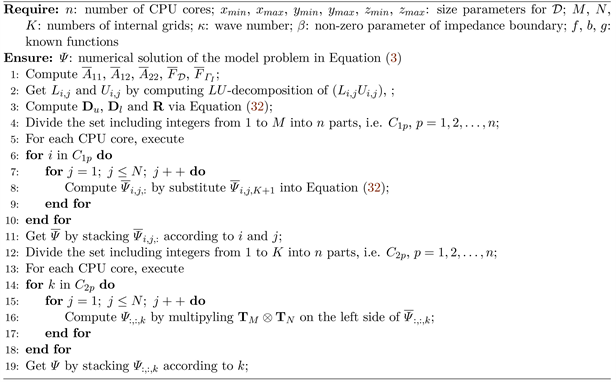
We notice that the calculation process of $\bar{\Psi }$ via Equation (32) is independent of i and j. Meanwhile, due to the feature of coefficient matrix and the sequence of components of $\bar{\Psi }$ , $\Psi =\left(T_M\otimes T_N\otimes I_K\right)\bar{\Psi }$ can be calculated separately with respect to k. Therefore, the steps computing $\bar{\Psi }$ and $\Psi$ can be processed in parallel. To summarize, Algorithm 1 demonstrates the steps of this fast algorithm.

6. Numerical Experiments

In this section, three numerical experiments with different coefficient $\beta$ are presented to demonstrate the validity, efficiency and applicability of the fast algorithm for Helmholtz impedance boundary value problem. We consider numerical experiments in the three-dimensional domain $\mathcal{D}=\left[\mathrm{0,1}\right]\times \left[\mathrm{0,1}\right]\times \left[\mathrm{0,1}\right]$ . All experiments are performed using MATLAB, and the BiCG method is adopted to solve the equations.

To test the performance of the fast algorithm, we offer the time of computing $\Psi$ from $\bar{\Psi }$ , error in $L_2$ and $L_{\infty }$ -norms. The definitions of error in $L_2$ and $L_{\infty }$ -norms are as follows

Algorithm 1. Fast algorithm based on discrete Fourier sine transform.

$\begin{array}{l}{e}_2={\left(\left(x_{\max }-x_{\min }\right)\left(y_{\max }-y_{\min }\right)\left(z_{\max }-z_{\min }\right){\left|{\Psi }^{*}-\Psi \right|}^2/\left(MNK\right)\right)}^{1/2}\mathrm{,}\\ e_M=\underset{}{{\displaystyle \max }}\left|{\Psi }^{*}-\Psi \right|\mathrm{,}\end{array}$

where ${\Psi }^{\mathrm{<mo>\; *\; </mo>}}$ and $\Psi$ are the exact solution and the numerical solution, respectively. Notice that $e_2$ should be ${\left(\frac{1}{MNK}{\left|{\Psi }^{\mathrm{<mo>\; *\; </mo>}}-\Psi \right|}^2\right)}^{1/2}$ due to the size of $\mathcal{D}$ . The convergence order of the algorithm is defined as

$\begin{array}{l}{\text{order}}_2=\frac{{\log }_2\left(e_2\left(h_n\right)/e_2\left(h_{n+1}\right)\right)}{{\log }_2\left(h_n/h_{n+1}\right)}\mathrm{,}\\ {\text{order}}_M=\frac{{\log }_2\left(e_M\left(h_n\right)/e_M\left(h_{n+1}\right)\right)}{{\log }_2\left(h_n/h_{n+1}\right)}\mathrm{,}\end{array}$ (38)

where $h_n$ represents the labels of different step size.

6.1. Example with $\beta =1$

This example tests the performance of the algorithm. When $\beta =1$ , the impedance boundary condition has the most general form. For the model problem (3) which has the exact solution

${\psi }^{\mathrm{<mo>\; *\; </mo>}}=\frac{1}{{\kappa }^2}\sin \left(3\pi x\right)\sin \left(\pi y\right)\sin \left(\kappa z\right)\mathrm{,}$ (39)

the model problem (3) can be derived as

$\begin{array}{l}\Delta \psi +{\kappa }^2\psi =-\frac{10{\pi }^2}{{\kappa }^2}\sin \left(3\pi x\right)\sin \left(\pi y\right)\sin \left(\kappa z\right)\mathrm{,}\text{in}\mathcal{D}\mathrm{,}\\ \psi =\frac{1}{{\kappa }^2}\sin \left(3\pi x\right)\sin \left(\pi y\right)\sin \left(\kappa z\right)\mathrm{,}\text{on}{\Gamma }_D\mathrm{,}\\ n\cdot \nabla \psi +\text{i}\kappa \beta \psi =\frac{1}{\kappa }\sin \left(3\pi x\right)\sin \left(\pi y\right){\text{e}}^{\text{i}\kappa z}\mathrm{,}\text{on}{\Gamma }_I\mathrm{.}\end{array}$ (40)

The computational errors, the time and memory consumption for different M are indicated in Table 1. With fewer grid points used ( $M=16,32$ ), the computational error between the numerical solution and the exact solution is only 10⁻⁷.

Table 1. Error, convergence rate, the time and memory consumption with $\kappa =3\pi$ and $\beta =1$ .

The convergence rate is calculated according to Equation (38) and is proved to be up to the fourth-order in $L_2$ and $L_{\infty }$ -norms. Moreover, the time and memory consumption are acceptable when the space complexity is $\mathcal{O}\left(M^3\right)$ . Figure 2 demonstrates the real part and imaginary part of numerical solution $\Psi$ . It can be seen that the imaginary part of the numerical solution appears mainly on the impedance boundary.

6.2. Example with $\beta =0$

When $\beta =0$ , the impedance boundary condition is simplified to Neumann boundary condition. In this case, the model problem (3) with the exact solution ${\psi }^{\mathrm{<mo>\; *\; </mo>}}$ in Equation (39) becomes the following

$\begin{array}{l}\Delta \psi +{\kappa }^2\psi =-\frac{10{\pi }^2}{{\kappa }^2}\sin \left(3\pi x\right)\sin \left(\pi y\right)\sin \left(\kappa z\right)\mathrm{,}\text{in}\mathcal{D}\mathrm{,}\\ \psi =\frac{1}{{\kappa }^2}\sin \left(3\pi x\right)\sin \left(\pi y\right)\sin \left(\kappa z\right)\mathrm{,}\text{on}{\Gamma }_D\mathrm{,}\\ n\cdot \nabla \psi =\frac{1}{\kappa }\sin \left(3\pi x\right)\sin \left(\pi y\right)\cos \left(\kappa z\right)\mathrm{,}\text{on}{\Gamma }_I\mathrm{.}\end{array}$ (41)

The convergence rate and some measures of the algorithm’s performance are shown in Table 2. With the Neumann boundary condition, the fast algorithm proposed in this paper still reach the convergence rate of the fourth order. Due to the simplification of the boundary conditions, the memory consumption and the time consumption of solving $\Psi$ have fallen by almost half compared with the case $\beta =1$ . The numerical solution and the error $\Psi -{\psi }_{\mathrm{<mo>\; :\; </mo>,\; <mo>\; :\; </mo>,\; <mo>\; :\; </mo>}}^{\mathrm{<mo>\; *\; </mo>}}$ are given in Figure 3. Since $\beta =0$ , both the numerical and exact solutions are real numbers. When $\kappa =7\pi$ and $M=256$ , the error is only 10⁻¹⁰, which shows that the algorithm also has good applicability to Neumann boundary condition.

6.3. Example with $\beta =-1$

The case of large wave numbers (or high frequency) is always a challenge for

Figure 2. Numerical solution $\Psi$ with $\kappa =3\pi$ and $M=256$ : Real part (left). Imaginary part (right).

Figure 3. Numerical solution $\Psi$ (left) and error (right) with $\kappa =7\pi$ and $M=256$ .

Table 2. Error, convergence rate, the time and memory consumption with $\kappa =7\pi$ and $\beta =0$ .

solving Helmholtz boundary value problem. In this example, we consider the model problem (3) when $\beta =-1$ and $\kappa =15\pi ,31\pi ,63\pi$ . With exact solution in Equation (39), the model problem can easily be derived. Assuming the velocity of sound wave is $c=340\text{m}/\text{s}$ , so the frequency is $f=c\kappa /2\pi =2550\text{Hz}$ , 5270 Hz and 10,710 Hz, respectively. Figure 4 illustrates the fitting lines between $\log \left(\text{Error}\right)$ and step h when $\kappa =15\pi$ . The slopes of the fitting lines represent the convergence rate according to Equation (38) and are 4.295 and 4.273, respectively.

When $\kappa =15\pi ,31\pi$ and $63\pi$ , the error of the numerical solution are plotted in Figures 5-7, respectively. It can be found that the Helmholtz equation is highly oscillatory with large wave numbers. With the wave number increasing, the error of both real part and imaginary part also increases, but it is still in the acceptable range. Furthermore, though the numerical solution has strong oscillation, the boundary between wave and wave is very clear. It shows that the algorithm has high resistance to “Pollution effect” in the case of large wave numbers.

Figure 4. log-log graph of $\log \left(h\right)$ and $\log \left(\text{Error}\right)$ with $\kappa =15\pi$ (i.e. $f=2550\text{Hz}$ ).

Figure 5. Error $\Psi -{\psi }_{\mathrm{<mo>\; :\; </mo>,\; <mo>\; :\; </mo>,\; <mo>\; :\; </mo>}}^{\mathrm{<mo>\; *\; </mo>}}$ with $\kappa =15\pi$ and $M=256$ : Real part (left). Imaginary part (right).

Figure 6. Error $\Psi -{\psi }_{\mathrm{<mo>\; :\; </mo>,\; <mo>\; :\; </mo>,\; <mo>\; :\; </mo>}}^{\mathrm{<mo>\; *\; </mo>}}$ with $\kappa =31\pi$ and $M=256$ : Real part (left). Imaginary part (right).

Figure 7. Error $\Psi -{\psi }_{\mathrm{<mo>\; :\; </mo>,\; <mo>\; :\; </mo>,\; <mo>\; :\; </mo>}}^{\mathrm{<mo>\; *\; </mo>}}$ with $\kappa =63\pi$ and $M=256$ : Real part (left). Imaginary part (right).

7. Conclusions and Suggestions

A fast high-order algorithm based on compact finite difference schemes is purposed to solve three-dimensional Helmholtz impedance boundary value problems. By using the discrete Fourier sine transform and forward Gaussian elimination, the large block tridiagonal linear systems derived from the original model problem is reduced to several independent smaller systems. Moreover, according to the arrangement format of the coefficient matrix, we parallelize the calculation program to further reduce the time consumption.

Numerical examples with impedance and Neumann boundary conditions are considered to verify the effectiveness and accuracy of the algorithm. Results dedicate that the algorithm achieves fourth-order convergence rate in $L_2$ and $L_{\infty }$ -norms, and consumes less time and memory. It has certain application and popularization value in engineering practice.

In the future, higher-order compact difference schemes can be derived for the three-dimensional Helmholtz boundary value problems with more complex boundary conditions, e.g. electromagnetic scattering and seismology. In that case, the algorithm can be modified and adopted to reduce the consumption of solving, including time cost and memory cost.

Acknowledgements

This research was funded by Fundamental Research Funds for the Central Universities (No.2021MS115).

Conflicts of Interest

The authors declare no conflicts of interest regarding the publication of this paper.

References

[1]	Kuo, C.W., Veltin, J. and McLaughlin, D.K. (2014) Acoustic Measurements of Models of Military Style Supersonic Nozzle Jets. Chinese Journal of Aeronautics, Chinese Journal of Aeronautics, 27, 23-33. https://doi.org/10.1016/j.cja.2013.12.006
[2]	Altmann, J. (2004) Acoustic and Seismic Signals of Heavy Military Vehicles for Co-Operative Verification. Journal of Sound and Vibration, 273, 713-740. https://doi.org/10.1016/j.jsv.2003.05.002
[3]	Sarvazyan, A.P., Urban, M.W. and Greenleaf (2013) Acoustic Waves in Medical Imaging and Diagnostics. Ultrasound in Medicine & Biology, 39, 1133-1146. https://doi.org/10.1016/j.ultrasmedbio.2013.02.006
[4]	Hughes-Riley, T. and Dias, T. (2018) Developing an Acoustic Sensing Yarn for Health Surveillance in a Military Setting. Sensors, 18, 1590. https://doi.org/10.3390/s18051590
[5]	Marshall, A. and Boussakta, S. (2007) Signal Analysis of Medical Acoustic Sounds with Applications to Chest Medicine. Journal of the Franklin Institute, 344, 230-242. https://doi.org/10.1016/j.jfranklin.2006.08.003
[6]	Behnia, A., Chai, H.K. and Shiotani, T. (2014) Advanced Structural Health Monitoring of Concrete Structures with the Aid of Acoustic Emission. Construction and Building Materials, 65, 282-302. https://doi.org/10.1016/j.conbuildmat.2014.04.103
[7]	He, C., Ni, X., et al. (2016) Acoustic Topological Insulator and Robust One-Way Sound Transport. Nature Physics, 12, 1124-1129. https://doi.org/10.1038/nphys3867
[8]	Chiatti, G., Chiavola, O. and Palmieri, F. (2017) A Vibration and Acoustic Characteristics of a City-Car Engine Fueled with Biodiesel Blends. Journal of Physical Society of Japan, 85, 664-670. https://doi.org/10.1016/j.apenergy.2016.10.119
[9]	Schelkunoff, S.A. (1938) The Impedance Concept and Its Application to Problems of Reflection, Refraction, Shielding and Power Absorption. Bell System Technical Journal, 17, 17-48. https://doi.org/10.1002/j.1538-7305.1938.tb00774.x
[10]	Shchukin, A.N. (1940) Propagation of Radio Waves. Svyazizdat, Moscow.
[11]	Leontovich, M.A. (1944) Methods of Solution for Problems of Electromagnetic Waves Propagation along the Earth Surface. Bulletin of the Academy of Sciences of the USSR. Physical Series, 8, 1622.
[12]	Leontovich, M. (1948) Approximate Boundary Conditions for Electromagnetic Field on the Surface of Conducting Bodies. In: Vvedenskii, B.A., Ed., Investigations on Propagation of Radio Waves, AN SSSR, Moscow, 5-10.
[13]	Alpert, Y.L. (1940) To the Problem of Electromagnetic Waves Propagation in Tubes. Journal of Technical Physics, 10, 1358-1364.
[14]	Zhang, X., Hu, X., Gong, H., Zhang, J., Lv, Z. and Hong, W. (2020) Experimental Study on the Impact Sound Insulation of Cross Laminated Timber and Timber-Concrete Composite Floors. Applied Acoustics, 161, Article ID: 107173. https://doi.org/10.1016/j.apacoust.2019.107173
[15]	Calleri, C., Astolfi, A., et al. (2019) Characterization of the Sound Insulation Properties of a Two-Layers Lightweight Concrete Innovative Façade, Applied Acoustics, 145, 267-277. https://doi.org/10.1016/j.apacoust.2018.10.003
[16]	Tsirigoti, D., Giarma, C. and Tsikaloudaki, K. (2020) Indoor Acoustic Comfort Provided by an Innovative Preconstructed Wall Module: Sound Insulation Performance Analysis. Sustainability, 12, 8666. https://doi.org/10.3390/su12208666
[17]	Kuo, S.M. and Tsai, J. (1994) Residual Noise Shaping Technique for Active Noise Control Systems. The Journal of the Acoustical Society of America, 95, 1665-1668. https://doi.org/10.1121/1.408555
[18]	Bodson, M., Jensen, J. and Douglas, S. (2001) Active Noise Control for Periodic Disturbances. IEEE Transactions on Control Systems Technology, 9, 200-205. https://doi.org/10.1109/87.896760
[19]	Sagartzazu, X., Hervella-Nieto, L. and Pagalday, J.M. (2008) Review in Sound Absorbing Materials. Archives of Computational Methods in Engineering, 15, 311-342. https://doi.org/10.1007/s11831-008-9022-1
[20]	Xia, B. and Yu, D. (2012) Modified Sub-Interval Perturbation Finite Element Method for 2D Acoustic Field Prediction with Large Uncertain-But-Bounded Parameters. Journal of Sound and Vibration, 311, 3774-3790. https://doi.org/10.1016/j.jsv.2012.03.024
[21]	Xia, B. and Yu, D. (2012) Interval Analysis of Acoustic Field with Uncertain-But-Bounded Parameters. Computers & Structures, 112-113, 235-244. https://doi.org/10.1016/j.compstruc.2012.08.010
[22]	Babuška, I.M. and Sauter, S.A. (1997) Is the Pollution Effect of the FEM Avoidable for the Helmholtz Equation Considering High Wave Numbers? SIAM Journal on Numerical Analysis, 34, 2392-2423. https://doi.org/10.1137/S0036142994269186
[23]	Lorca, J.P.L., Beams, N., Beecroft, D. and Gillman, A. (2023) An Iterative Solver for the HPS Discretization Applied to Three Dimensional Helmholtz Problems.
[24]	Galkowski, J., Lafontaine, D., Spence, E.A. and Wunsch, J. (2022) The hp-FEM Applied to the Helmholtz Equation with PML Truncation Does Not Suffer from the Pollution Effect.
[25]	Spence, E.A. (2022) A Simple Proof That the hp-FEM Does Not Suffer from the Pollution Effect for the Constant-Coefficient Full-Space Helmholtz Equation. Advances in Computational Mathematics, 49, Article No. 27. https://doi.org/10.1007/s10444-023-10025-3
[26]	Kumar, N. and Dubey, R.K. (2019) Development of a New Sixth Order Accurate Compact Scheme for Two and Three Dimensional Helmholtz Equation.
[27]	Feng, Q., Han, B. and Michelle, M. (2023) Sixth Order Compact Finite Difference Method for 2D Helmholtz Equations with Singular Sources and Reduced Pollution Effect.
[28]	An, S., Gu, G. and Zhao, M. (2018) A Fast High Order Algorithm for 3D Helmholtz Equation with Dirichlet Boundary. Applied and Computational Mathematics, 7, 180-187. https://doi.org/10.11648/j.acm.20180704.11
[29]	Zhu, N. and Zhao, M. (2018) A Fast Fourth-Order Method for 3D Helmholtz Equation with Neumann Boundary. American Journal of Computational Mathematics, 8, 222-232. https://doi.org/10.4236/ajcm.2018.83018