1. Introduction
The mathematical field of Graph Theory first came into prominence after Euler published his paper on the Königsberg 7 bridges problem. Following that, numerous mathematicians expanded the field and created new classifications of graphs as well as new problems, such as the famous 4 color problem (which is a special case of the T-coloring of graphs). There have long been many real world applications from graph theory, such as radio transmission and map coloring. The issue that arises with these types of problems is a conflict of organization. Vertices must be carefully positioned so that edge crossing can be avoided under certain circumstances, and with increasingly complicated situations, comes a need for greater detail and precision in its graph labeling. For example, in the case of radio transmissions, signals within close vicinity cannot overlap and therefore must be assigned to avoid conflicts. Each radio station is assigned a unique radio frequency. The closer the locations for radio stations are, the greater the risk for signal interference. To solve this, our paper will signify radio stations as vertices and radio frequencies as labels and make it into a graphing problem.
The problem of T-coloring of graphs has long been heavily researched. Starting in the 1980s, a new application of this problem was the issue of channel frequency assignment [2] [3] [4] [5]. Another wave of research on this topic began in 1990s, with an effort to more efficiently assign radio channels by using non negative integers, whereas channels at close distances receive frequencies further apart in value than channels at far apart distances [6] [7] [8] [9]. This should prevent signal interference between radio stations close to each other. In particular, Griggs and Yeh’s work in [6] on graph labeling with a condition at distance 2 vertices is of great importance. They proposed a new way to label a graph. Given a graph
and a positive integer d, an
labeling of G is a real-valued function
such that, for any two vertices x and y in G,
The
-labeling number, denoted by
, is the smallest integer m such that G has an
-labeling
. When
, Griggs and Yeh proved that
, where
is the maximum degree of G. Their result was later improved by Král’ and Skrekovski [10], who proved
when
.
Recently, Yeh continued his previous work in [6]: instead of assigning a single number to a vertex, he assigned a set of numbers to each vertex. Let [k] be
the integer set
and
be the set of all n-subsets of [k]. Given
a positive integer k and non-negative integers
and
with
, an
-labeling is a function
such that, for any two vertices x and y in G,
where
is the defined set difference. Figure 1 is an illustration of the above definition.
The smallest k satisfying the above definition is called the
-labeling number of G and denoted by
. In particular, when
,
is denoted by
for short. Yeh applied this idea and obtained
![]()
Figure 1. Illustration of
-labeling.
the exact value of
for several types of graphs: trees, wheels, the square lattice, the hexagonal lattice, and the triangular lattice. For the cycle graphs
, Yeh has completely solved the problem for
. (Note: There was a typo in Corollary 3.5 [6], where the results there should be read only for
.) For the general cases when
, Yeh proved that
In this paper, we will expand on Yeh’s work for
with
on the following uncovered cases:
1)
with
;
2)
with
.
For the rest of this paper, we will refer any of the above unstudied cases as an uncovered case. Our goal is to fill in the gaps and find out the
for the uncovered cases.
2.
for
and
Yeh [6] proved that, if G is a graph with diameter 2 and order m, then
. Since both
and
have diameter 2, as shown in Figure 2, the following is a direct consequence of Yeh’s observation.
Lemma 1
and
.
3. Proving Lower Bound for
for Uncovered Cases
In order to obtain a general formula for the lower bound of
for uncovered m values given in Section 1, we first introduce the following lemma:
3.1. Upper Bound for Label Repetition
Lemma 2 In any
-labeling of
, no label can be used more than
times.
Proof. We will prove the lemma by contradiction. Let
, where
is adjacent to
for each i with
, shown in Figure 3.
![]()
Figure 2. Cyclic graphs for
and
.
Let
. Without loss of generality, we may assume that a label “
” is
assigned to
and is used
times in an
-labeling of
. Let
be the distance between a pair of adjacent “
” labels in the cyclic order (Please refer to Figure 3). The total distance is m because there are m vertices:
This implies that
Thus the smallest
must be either 1 or 2; in other words, there are two vertices of
with distance at most two receiving the same label “
”. This contradicts the distance labeling condition for
, and thus Lemma 2 is proved. 
3.2. Lower Bound for
for All Uncovered Cases
Theorem 1 For all integers m and n with
,
where
.
Proof. In any
-labeling of
, each vertex receives m labels. So there are together mn labels (counting the repetition of each label). By Lemma 2, each distinct label can only be repeatedly used at most p times. This implies that there are at least mn/p distinct labels. Also labels can start from 0 and
is the largest label, we have
. 
4.
for
We find all values for
.
Theorem 2
Proof. By Yeh’s work [6] and Lemma 1, we only need to prove the theorem for the uncovered cases when
. By Theorem 1,
On the other hand, we can prove that the above lower bounds are also upper bounds by constructing actual label assignments.
For
, the following label assignment meets the
-labeling requirement. (Each block of three labels is assigned to a vertex of
in the cyclic order. Similar label assignments are applied for other uncovered cases
below.)
0 1 2 || 3 4 5 || 6 7 8 || 9 10 0 || 1 2 3 || 4 5 6 || 7 8 9 ||
This indicates:
For
, the following label assignment meets the
-labeling requirement:
0 1 2 || 3 4 5 || 6 7 8 || 9 10 11 || 0 1 2 || 3 4 5 || 6 7 8 || 9 10 11 ||
This indicates:
For
, the following label assignment meets the
-labeling requirement:
0 1 2 || 3 4 5 || 6 7 8 || 9 10 0 || 1 2 3 || 4 5 6 || 7 8 9 || 10 0 1 || 2 3 4 || 5 6 7 || 8 9 10 ||
This indicates:
For
, the following label assignment meets the
-labeling requirement:
0 1 2 || 3 4 5 || 6 7 8 || 9 10 0 || 1 2 3 || 4 5 6 || 7 8 9 || 10 0 1 || 2 3 4 || 5 6 7 || 8 9 10 || 0 1 2 || 3 4 5 || 6 7 8 ||
This indicates:
For
, the following label assignment meets the
-labeling requirement:
0 1 2 || 3 4 5 || 6 7 8 || 9 10 0 || 1 2 3 || 4 5 6 || 7 8 9 || 10 0 1 || 2 3 4 || 5 6 7 || 8 9 10 || 0 1 2 || 3 4 5 || 6 7 8 || 9 10 0 || 3 4 5 || 6 7 8 ||
This indicates:
By combining the upper and lower bounds together, we conclude that
when
and that
. 
5.
for
In this section, we find all values for
.
Theorem 3
Proof. By Yeh’s work [6] and Lemma 1, we only need to prove the theorem for the uncovered cases when
. By Theorem 1,
On the other hand, we can prove that the above lower bounds are also upper bounds by constructing actual label assignments.
For
, the following label assignment meets the
-labeling requirement:
0 1 2 3 || 4 5 6 7 || 8 9 10 11 || 12 13 0 1 || 2 3 4 5 || 6 7 8 9 || 10 11 12 13 ||
This indicates:
For
, the following label assignment meets the
-labeling requirement:
0 1 2 3 || 4 5 6 7 || 8 9 10 11 || 12 13 14 15 || 0 1 2 3 || 4 5 6 7 || 8 9 10 11 || 12 13 14 15 ||
This indicates:
For
, the following label assignment meets the
-labeling requirement:
0 1 2 3 || 4 5 6 7 || 8 9 10 11 || 12 13 0 1 || 2 3 4 5 || 6 7 8 9 || 10 11 12 13 || 0 1 2 3 || 4 5 6 7 || 8 9 10 11 ||
This indicates:
For
, the following label assignment meets the
-labeling requirement:
0 1 2 3 || 4 5 6 7 || 8 9 10 11 || 12 13 14 0 || 1 2 3 4 || 5 6 7 8 || 9 10 11 12 || 13 14 0 1 || 2 3 4 5 || 6 7 8 9 || 10 11 12 13 ||
This indicates:
For
, the following label assignment meets the
-labeling requirement:
0 1 2 3 || 4 5 6 7 || 8 9 10 11 || 12 13 0 1 || 2 3 4 5 || 6 7 8 9 || 10 11 12 13 || 0 1 2 3 || 4 5 6 7 || 8 9 10 11 || 12 13 0 1 || 2 3 4 5 || 6 7 8 9 || 10 11 12 13 ||
This indicates:
For
, the following label assignment meets the
-labeling requirement:
0 1 2 3 || 4 5 6 7 || 8 9 10 11 || 12 13 0 1 || 2 3 4 5 || 6 7 8 9 || 10 11 12 13 || 0 1 2 3 || 4 5 6 7 || 8 9 10 11 || 12 13 0 1 || 2 3 4 5 || 6 7 8 9 || 10 11 12 13 || || 0 1 2 3 || 4 5 6 7 || 8 9 10 11 ||
This indicates:
For
, the following label assignment meets the
-labeling requirement:
0 1 2 3 || 4 5 6 7 || 8 9 10 11 || 12 13 0 1 || 2 3 4 5 || 6 7 8 9 || 10 11 12 13 || 0 1 2 3 || 4 5 6 7 || 8 9 10 11 || 12 13 0 1 || 2 3 4 5 || 6 7 8 9 || 10 11 12 13 || || 0 1 2 3 || 4 5 6 7 || 8 9 10 11 || 12 13 0 1 || 4 5 6 7 || 8 9 10 11 ||
This indicates:
For
, the following label assignment meets the
-labeling requirement:
0 1 2 3 || 4 5 6 7 || 8 9 10 11 || 12 13 0 1 || 2 3 4 5 || 6 7 8 9 || 10 11 12 13 || 0 1 2 3 || 4 5 6 7 || 8 9 10 11 || 12 13 0 1 || 2 3 4 5 || 6 7 8 9 || 10 11 12 13 || 0 1 2 3 || 4 5 6 7 || 8 9 10 11 || 12 13 2 3 || 4 5 6 7 || 8 9 10 11 || 12 13 2 3 || 4 5 6 7 || 8 9 10 11 ||
This indicates:
Here is the general process of label assignment for
and
, whose complete data set is: 0 1 2 3 4 5 6 7 8 9 10 11 12 13.
1) We iterate this data set repeatedly by combining 4 labels in a group and assigning this group to one node.
2) This process continues until we finish the 23rd node.
Please note that there is something special with the label assignment for
. For the last two repetitions of the data set, the “0” and “1” were taken out, indicated by the bold numbers. This is to avoid violation of
-labeling requirements. This algorithm will be explained in detail in the next section.
By combining the upper and lower bounds together, we conclude that
when
,
and
. 
There is not a general formula for the uncovered cases. For any given n value, we need to work on each corresponding uncovered m value individually.
6. Algorithm for Finding Upper Bound for All Uncovered Cases
We have proven the lower bound for all the uncovered cases. In this section, we will work on the upper bound. We will use the prove-by-construction method and provide a general algorithm to find label assignment for all the uncovered cases based on the proved lower bound. The finding of such label assignment gives an upper bound to
.
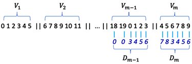
6.1. Sample Case of
We will use the following case to illustrate how we will construct the label assignment for all the vertices based on the lower bound.
(number of labels per vertex)
(number of vertices)
The lower bound is calculated according to Section 3.2:
(max number of repetitions per label)
(lower bound of
for
)
Data set available for the labels to be used for each vertex: 0, 1, 2, 3, … 16, 17, 18, 19.
Initial label assignment:
0 1 2 3 4 5 || 6 7 8 9 10 11 || 12 13 14 15 16 17 || 18 19 0 1 2 3 || 4 5 6 7 8 9 || 10 11 12 13 14 15 || 16 17 18 19 0 1 || 2 3 4 5 6 7 || 8 9 10 11 12 13 || 14 15 16 17 18 19 || 0 1 2 3 4 5 || 6 7 8 9 10 11 || 12 13 14 15 16 17 || 18 19 0 1 2 3 || 4 5 6 7 8 9 || 10 11 12 13 14 15 || 16 17 18 19 0 1 || 2 3 4 5 6 7 || 8 9 10 11 12 13 || 14 15 16 17 18 19 || 0 1 2 3 4 5 || 6 7 8 9 10 11 || 12 13 14 15 16 17 || 18 19 0 1 2 3 || 4 5 6 7 8 9 || 10 11 12 13 14 15 || 16 17 18 19 0 1 || 2 3 4 5 6 7 || 8 9 10 11 12 13 || 14 15 16 17 18 19 || 0 1 2 3 4 5 || 6 7 8 9 10 11 || 12 13 14 15 16 17 || 18 19 0 1 2 3 || 4 5 6 7 8 9 ||
Initial label assignment for the first and last two vertices:
Violations found:
• 4 labels (0, 1, 2, 3) in
are overlapping with that of
: distance 2 type of violation;
• 2 labels (4, 5) in
are overlapping with that of
: distance 1 type of violation, which requires more corrective shifts towards the left;
• 4 labels (6, 7, 8, 9) in
are overlapping with that of
: distance 2 type of violation.
Corrections:
(1) Use two arrays
and
to record the minimum displacement needed for each label position in
and
, in case a corrective shift (to the left) is needed for a violation.
indicates no violation for the ith position in
.
indicates no violation for the ith position in
.
(2) Assignment of displacement values for
:
•
because
, and 18 does not overlap with any labels in
;
•
because
, and 19 does not overlap with any labels in
;
•
because
, and 0 overlaps with a label in
; 0 needs to shift at least 3 positions towards left to resolve this violation;
•
because
, and 1 overlaps with a label in
; 1 needs to shift at least 4 positions towards left to resolve this violation;
•
because
, and 2 overlaps with a label in
; 2 needs to shift at least 5 positions towards left to resolve this violation;
•
because
, and 3 overlaps with a label in
; 3 needs to shift at least 6 positions towards left to resolve this violation;
(3) Assignment of displacement values for
:
•
because
, and 4 overlaps with a label in
; 4 needs to shift at least 7 positions towards left to resolve this distance 1 type of violation;
•
because
, and 5 overlaps with a label in
; 5 needs to shift at least 8 positions towards left to resolve this distance 1 type of violation;
•
because
, and 6 overlaps with a label in
; 6 needs to shift at least 3 positions towards left to resolve this violation;
•
because
, and 7 overlaps with a label in
; 7 needs to shift at least 4 positions towards left to resolve this violation;
•
because
, and 8 overlaps with a label in
; 8 needs to shift at least 5 positions towards left to resolve this violation;
•
because
, and 9 overlaps with a label in
; 9 needs to shift at least 6 positions towards left to resolve this violation;
(4)
for all i.
(5) Use of
for corrections.
In order to accomplish the corrective displacement for the above labels, we will shift every label
positions toward the left for the last two vertices. This indicates that we need to create
extra positions from the previous vertices. A divide-and-conquer strategy is used.
In this case, a complete data set has 20 numbers (0, 1, 2, 3, …, 16, 17, 18, 19) available to use for the label assignment. We can safely remove 2 numbers from each data set to help with the shift-left task, because three consecutive vertices need a total of 18 different labels to avoid violation of
rules. These two numbers can be any number from 0 to 19. For example,
(6.1)
Without loss of generality, we will remove the first two numbers (0, 1) from each of the last 4 data sets as indicated in (6.1), creating a total of 8 extra positions for the later data to fill in. This will satisfy the
required for resolving violations.
New label assignment:
0 1 2 3 4 5 || 6 7 8 9 10 11 || 12 13 14 15 16 17 || 18 19 0 1 2 3 || 4 5 6 7 8 9 || 10 11 12 13 14 15 || 16 17 18 19 0 1 || 2 3 4 5 6 7 || 8 9 10 11 12 13 || 14 15 16 17 18 19 || 0 1 2 3 4 5 || 6 7 8 9 10 11 || 12 13 14 15 16 17 || 18 19 0 1 2 3 || 4 5 6 7 8 9 || 10 11 12 13 14 15 || 16 17 18 19 0 1 || 2 3 4 5 6 7 || 8 9 10 11 12 13 || 14 15 16 17 18 19 || 0 1 2 3 4 5 || 6 7 8 9 10 11 || 12 13 14 15 16 17 || 18 19 * * 2 3 4 5 || 6 7 8 9 10 11 || 12 13 14 15 16 17 || 18 19 * * 2 3 4 5 || 6 7 8 9 10 11 || 12 13 14 15 16 17 || 18 19 * * 2 3 4 5 || 6 7 8 9 10 11 || 12 13 14 15 16 17 || 18 19 * * 2 3 4 5 || 6 7 8 9 10 11 || 12 13 14 15 16 17 ||
New label assignment for the first and last two vertices:
0 1 2 3 4 5 || 6 7 8 9 10 11 || … || 6 7 8 9 10 11 || 12 13 14 15 16 17
We now have no more violations! Please note the spots marked with * within the groups of bold numbers. These are the positions which were originally occupied by 0 s and 1 s.
Therefore, we successfully constructed the label assignment with the lower bound. This means that the lower bound is also the upper bound for n = 6 with m = 35. Thus, we have
.
6.2. General Algorithm for Finding Label Assignment Based on Lower Bound
In this section, we provide a general algorithm to find the label assignment for the purpose of finding the upper bound of
with
for the following uncovered cases:
(6.2)
Number of uncovered vertices:
For each m value listed in (6.2):
(1) Calculate the following parameters:
; p is the maximum number of repetitions per label.
; L is the lower bound for
.
; r is the number of labels which can be safely removed from
each data set without violation of
.
(2) Initialize index, whose value ranges from 0 to L; One complete data set runs from 0 to L.
(3) Initial label assignment:
For each of the m vertices
For each of the n positions available for labels
Assign a proper index to each label position;
Increase index by 1;
If (index > L) reset index =0;
Complexity:
.
(4) Print out the initial label assignment for the first and last two vertices:
.
Complexity: 4n.
(5) Check possible violation of requirement for
: we only need to check
against
, and
against both
and
.
Use two arrays
and
to record the minimum displacement needed for each label position in
and
, in case a corrective shift (to the left) is needed for a violation.
indicates no violation for theith position in
.
indicates no violation for the ith position in
.
Step 1: Compare each label of
with that of
. Any overlapped labeling indicates a violation of distance 2 type, and the corresponding
will be recorded. Complexity: n2.
Step 2: Compare each label of
with that of
. Any overlapped labeling indicates a violation of distance 1 type which requires more corrective shifts toward left, and the corresponding
will be recorded. Complexity: n2.
Step 3: Compare each label of
with that of
. Any overlapped labeling indicates a violation of distance 2 type, and the corresponding
will be recorded. Complexity: n2.
Step 4:
. This is the minimum corrective displacement needed to shift every label of the last two vertices toward left to avoid
violation; Complexity:
.
(6) If
, no violations; label assignment is done for this m value.
(7) If
, adjust label assignment:
;
For the first
data set, use index values from 0 to L to assign labels;
For the rest of data set, only use index values from r to L to assign labels;
Complexity:
.
(8) Print out the updated label assignment for the first and last two vertices:
.
Complexity: 4n.
(9) Check possible violation of requirement for
:
We only need to check
against
, and
against both
and
. Use similar methods described in step 1 to step 4 listed above.
Complexity:
.
(10) If
, no violations; the updated label assignment works for this m value. Otherwise, print out error message: Failed label assignment for
.
6.3. Runtime and Complexity
From Section 6.2, we can figure out that the runtime complexity to calculate
and find a no-violation cyclic label assignment for a given pair of
is:
(6.3)
Applying (6.3), the runtime complexity to calculate
and find a no-violation cyclic label assignment for all the uncovered m values with a given n value is:
(6.4)
The complexity of (6.4) is in the order of n3.
When we run the program for all the n values from 3 to N, the runtime complexity is:
(6.5)
The complexity of (6.5) is in the order of
.
Laptop configuration: 4 core, 8 thread, i7, 8 GB ram, 100 GB hard drive.
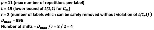
Runtime and size of output file when only the label assignment for the first and last two vertices were printed:
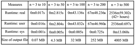
Runtime and size of output file when label assignment for all the vertices were printed:
6.4. Results
We tested our algorithm for every n value from 3 to 500 and every case was successful. A sample case for
is listed below:
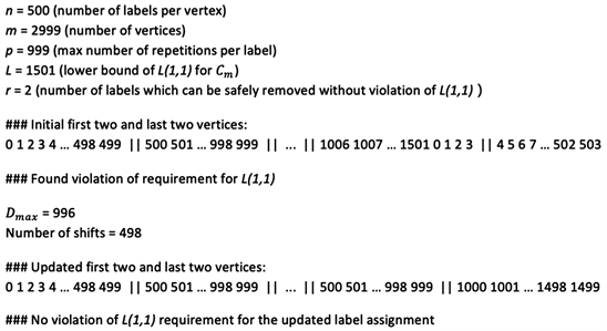
Our results demonstrate that we can use the lower bound to construct the label assignment without violation of
for n values up to 500. This indicates the upper bound is the same as the lower bound. Therefore, we have:
Conjecture: For all integers m andn with m, n ≥ 3, the smallest possible value for the largest label needed is given by
(6.6)
where n is the number of labels per vertex, m is the number of vertices, and
is the maximum number of repetitions per label.
We did not continue with n values bigger than 500 in our code, because the output file size went over 4 GB with
when we only print out the first and last two vertices, and the output file size went over 22 GB with
when we print out label assignment for every vertex. Practically,
is large enough to demonstrate the feasibility of our algorithm, and the correctness of (6.6).
7. Conclusions
In this paper, we studied the label assignment for cycle graphs, and we focused on the
for the m values which were left uncovered by [1] due to their case-by-case complexities. We achieved a lower bound, expressed by Theorem 1, for all the uncovered m values. Moreover, based on the lower bound, we developed an algorithm in Section 6.2 to construct a no-violation label assignment for all vertices in order to find the corresponding upper bound. We ran every single case for
and obtained successful label assignments.
Theoretically, our algorithm can be used for any
to find a feasible label assignment. Anybody interested in uncovered cases for
is welcome to verify the label assignment using our algorithm.