Analysis of State Homicide Rates Using Statistical Ranking and Selection Procedures

Anqi Wang, Gary C. McDonald

Department of Mathematics and Statistics, Oakland University, Rochester, MI, USA.

DOI: 10.4236/am.2022.137037                

Abstract

Nonparametric and parametric subset selection procedures are used in the analysis of state homicide rates (SHRs), for the year 2005 and years 2014-2020, to identify subsets of states that contain the “best” (lowest SHR) and “worst” (highest SHR) rates with a prescribed probability. A new Bayesian model is developed and applied to the SHR data and the results are contrasted with those obtained with the subset selection procedures. All analyses are applied within the context of a two-way block design.

Keywords

Homicide Rates Analysis Reporting System, Probability of a Correct Selection, Bayesian Inference, WinBugs, Additive Model, Tukey One-Degree-of-Freedom Test for Additivity

1. Introduction

The United States experienced its biggest one-year increase on record in homicides in 2020, according to new figures released by the F.B.I. There is no simple explanation for the steep rise. A number of key factors are driving the violence, including the economic and social toll taken by the pandemic and a sharp increase in gun purchases. However, how does the homicide rate appear before 2020? As reported in a Wall Street Journal article [1], “the rate of 6.5 homicides per 100,000 residents is the highest since 1997, but still below historic highs of the early 1990s”. This article further explores possible causes for the recent increasing trends in homicide rates.

This article focuses on the application of nonparametric (or distribution-free), parametric subset selection procedures and the Bayesian approach to analyze state homicide rate (SHR) data for the year 2005 and years 2014-2020. With the Bayesian approach, a probability distribution is derived over all possible permutations of the population means. Thus, the probability that any particular state is characterized by the largest (or smallest) mean can be easily obtained by appropriate summing of the permutation probabilities. The variability of SHRs is herein analyzed with advanced statistical techniques. While root causal analysis is also very important, it requires different investigative approaches.

The state homicide rate data is obtained from CDC: https://www.cdc.gov/nchs/pressroom/sosmap/homicide_mortality/homicide.htm

There is an existing gap from the year 2005 to 2014 while addressing the data. The rate of 0.00 is not actually zero since we kept 2 decimal points for the data.

2. Formulation of Nonparametric Subset Selection Rules

The description of this selection rule will follow that given by Green and McDonald [2], Let Π₁, Π₂, ∙∙∙, Π_k be k(≥2) independent pupulations. The associated random variables, X_ij, j = 1, ∙∙∙, n; i = 1, ∙∙∙, k, are assumed independent and to have a continuous distribution F_j(x; θ_i) where θ_i belong to some interval Θ on the real line. The basic model assumption is that F_j(x; θ_i) is a stochastically increasing family of distributions for each j. The additive model of the following form is used:

$X_{ij}=\mu +{\theta }_i+{\beta }_j+{\epsilon }_{ij}$ (1)

where β_j indicates the particular block effect, θ_i indicates the population effect, and ε_ij is the random error. The distribution of ε_ij is any continuous distribution function F_j(x) with mean 0. The distribution of X_ij will be stochastically ordered in θ as it is a location parameter in Equation (1). So, for example, F_j(x) could be a normal distribution with mean 0 and standard deviation σ_j. The assumption of negligible interaction between population and block must be satisfied. Let θ_[i] denote the ith smallest unknown parameter, then for all x

$F_j\left(x;{\theta }_{\left[1\right]}\right)\ge F_j\left(x;{\theta }_{\left[2\right]}\right)\ge \cdots \ge F_j\left(x;{\theta }_{\left[k\right]}\right)$ (2)

where θ_[1] (θ_[k]) characterizes the best (worst) population.

Let R_ij denote the rank of the observation X_ij among X_1j, X_2j, ∙∙∙, X_kj. The variables R_ij take values from 1 to k. The selection procedures considered here are based on the rank sums, T_i = S_jR_ij, associated with Π_i, i = 1, ∙∙∙, k. The structure for this process is outlined in Table 1.

Any subset selection procedure based on the rank sums should have the property that the probability that a correct selection (CS) occurs, i.e., the worst population (or best population) is included in the selected subset, is bounded below by P^*(k⁻¹ < P^* < 1). That is, for a given selection rule R, the probability of a CS should satisfy the inequality,

$\underset{\Omega }{\inf }P\left(\text{CS}|\text{R}\right)\ge P^{*}$, (3)

where $\Omega =\left\{\theta =\left({\theta }_1,\cdots ,{\theta }_k\right):{\theta }_i\in \Theta ,i=1,\cdots ,k\right\}$. In some cases, as noted later, inequality may only hold on a subspace Ω' of Ω.

Table 1. Structure for determining ranks and rank sums.

The two selection rules for choosing a subset containing the worst population, as described in McDonald [3], are given by:

R₁: Select Π_i iff T_i ≥ max(T_j) – b₁

R₂: Select Π_i iff T_i > b₂.

Similarly, the two selection rules for choosing a subset containing the best population are given by:

R₃: Select Π_i iff T_i ≤ min(T_j) + b₃

R₄: Select Π_i iff T_i < b₄.

Note that the rules R₁ and R₂ could be written in the form that select Π_i iff T_i > b, where b is a stochastic quantity for R₁ and a deterministic quantity for R₂. A similar statement can be made for the rules R₃ and R₄.

As developed by McDonald [4] [5] [6], R₁ and R₃ are justified over a slippage space, Ω', where all parameters θ_i are equal with the possible exception of θ_[k] in case of rule R₁ or θ_[1] in case of rule R₃; and R₂ and R₄ are applicable over the entire parameter space. The constants b₁, b₃, and b₄ are chosen as small as possible and b₂ is chosen as large as possible preserving the probability goal. For large values of n, the selection rules are determined by the asymptotic formulae as described in McDonald [5] and are computed as:

$b_1=b_3=h{\left[nk\left(k+1\right)/6\right]}^{1/2}$, (4)

$b_2={\left[n\left(k^2-1\right)/12\right]}^{1/2}{\Phi }^{-1}\left(1-P^{*}\right)+n\left(k+1\right)/2$, (5)

$b_4=n\left(k+1\right)-b_2$, (6)

where the h-solution to be used in Equation (4) is given by:

${\displaystyle {\int }_{-\infty }^{\infty }{\Phi }^{k-1}\left(x+h\sqrt{2}\right)\varphi \left(x\right)\text{d}x}=P^{*}$. (7)

Here, Φ and $\varphi$ represent the standard normal cumulative distribution function (CDF) and probability density function (PDF), respectively.

Taking P^* to be particular confidence level, the h-solution is given in Table 1 of Gupta et al. [7], and can be used to determine the constants b₁ and b₃. The above integral can also be calculated to determine P^* for a given value of h, using a TI-83+ (or similar) calculator with numerical integration capability as shown in Green and McDonald [2]. The integral can be shown to be the probability that the maximum of U_i, i = 1, ∙∙∙, k, is less than h where the U_i are normally distributed random variables with zero means, unit variances, and covariance of 0.5 (see Gupta et al. [7]). With confidence level P^*, it can be asserted (using these selection rules) that the chosen subset of the populations contains the one characterized by θ_[k] (θ_[1]).

Since there is only one observation for each state for each year, there is no general test for additivity, i.e., lack of interaction between states and years. Tukey developed a one degree-of-freedom test for nonadditivity when there is a single observation per cell, as given here. This test is used to establish the plausibility of model (1) for a power transformation of the SHRs. Table 2 shows the Tukey one degree-of-freedom test for nonadditivity for the SHRs and for these rates raised to the 0.4 power. The test indicates significant evidence of interaction with the untransformed rates, and no significant evidence of interaction with the power transformation of the rates. The Tukey test is testing for interaction of the form $E\left(X_{ij}\right)=\mu +{\theta }_i+{\beta }_j+\lambda {\theta }_i{\beta }_j$. And the one degree of freedom test is given by testing for the one parameter λ. For the purpose of the nonparametric analyses to follow, the original SHR data will be used because ranks are invariant to monotone increasing transformations.

3. Nonparametric Subset Selection of States

The goal is now to choose a subset of the 50 states that can be asserted, with a specified confidence, to contain the state with the highest SHR (worst population), and similarly a state with the lowest SHR (best population) using the nonparametric ranking and selection procedures. Ranks k = 1, ∙∙∙, 50 are assigned to states for each of n = 8 years, with a rank of “1” being the state with the lowest SHR. Based on these ranks, the selection procedure for choosing a subset of the 50 states asserts that the best state (or worst state) is contained with a specified confidence level P^*.

Table 2. Tukey’s one degree-of-freedom test.

Similar to the structure as outlined in the second section, let R_ij denote the rank of the observation X_ij within the jth block. The variables R_ij take values from 1 to k and the selection procedure is based on the rank sums, $T_i={\displaystyle {\sum }_j{R}_{ij}}$, associated with Π_i, i = 1, ∙∙∙, k. In the case of ties, each tied state receives an average of their rank for that year. This is done for all 7 years. Ranks are then summed for each state and the rank sums T_i’s, are orderd. The selection rule constants are determined by the asymptotic formulae as described in the second section.

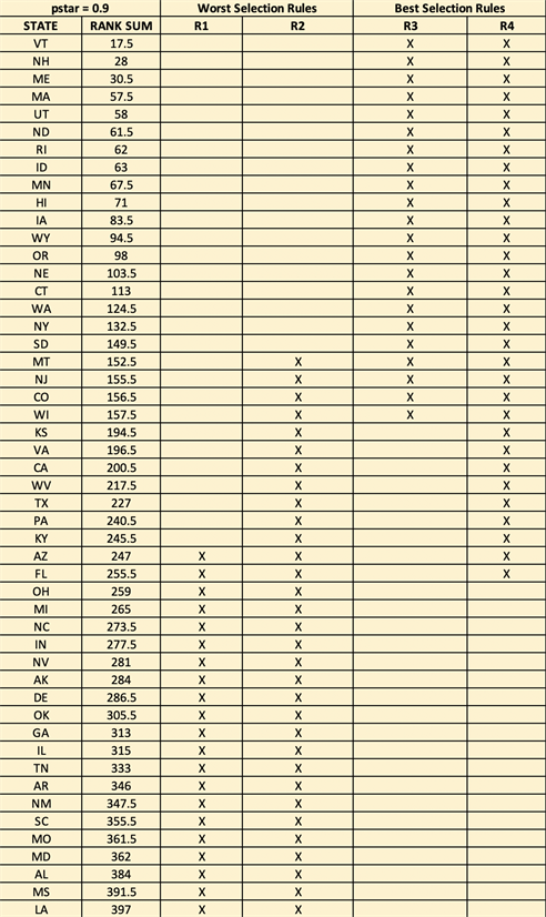
Taking P^* = 0.90, the h-solution as given in Table 1 of Gupta et al. [7], is h = 2.581. This can be used to determine the constants b₁ and b₃. Using n = 8, k = 50, and h = 2.581, we obtain b₁ = b₃ = 150.5. Since n = 8 is not a particularly large sample size, the asymptotic values are compared with simulated values as described in McDonald [8]. The simulated value would yield b₁ = b₃ = 148 vs. 150.5 using the asymptotic formula. The other two constants are calculated to be b₂ = 151.7 and b₄ = 256.3. The data yields max(T_j) = 397, and min(T_j) = 17.5. The choice of P^* = 0.90 is determined by the degree of assurance one wishes to have concerning the goal of the chosen subset of states. This is similar to the choice of the level of confidence, an analyst would have concerning a confidence interval for a population parameter, e.g., the mean or variance.

With confidence level P^* = 0.90, it can be asserted that the following subsets of states contain that one characterized by θ_[k]:

Rule R₁: Select the ith state iff T_i ≥ max(T_j) – 150.5 = 246.5. Twenty-one are chosen for “worst”.

Rule R₂: Select the ith state iff T_i > 151.7. Thirty-two are chosen for “worst”.

With the same 0.90 confidence level, it can be asserted that the following subset of states contain that one characterized by θ_[1]:

Rule R₃: Select the ith state iff T_i ≤ min(T_j) + 150.5 = 168.0. Twenty-two are chosen for “best”.

Rule R₄: Select the ith state iff T_i < 256.3. Thirty-one are chosen for “best”.

The identification of the specific states chosen with these four selection rules is given in Appendix B.

4. Parametric Subset Selection of States

In this section, a normal means parametric selection procedure will be used to contrast the inference with that of the nonparametric approach. This approach to subset selection was developed by Gupta [9]. With the additive model (1)

$E\left(X_{ij}\right)=\mu +{\theta }_i+{\beta }_j$ (8)

Letting ${\bar{X}}_i=\left({\displaystyle {\sum }_j{X}_{ij}}\right)/n$, then $E\left({\bar{X}}_i\right)=\mu +{\theta }_i+\left({\displaystyle {\sum }_j{\beta }_j}\right)/n$. Since the quantity $\mu +\left({\displaystyle {\sum }_j{\beta }_j}\right)/n$ is constant for all i, inference on the ordered θ_i can be efficiently based on the ordering of the means, ${\bar{X}}_i$.

The additive model (1) will be used with X_ij replaced with $f\left(X_{ij}\right)=X_{ij}^{0.4}$ based on the results given in Table 2. Here, the ε_ij are assumed independent identically distributed normal variates with mean 0 and standard deviation σ. Residual displays from a two-way additive analysis of variance (ANOVA) are given in Figure 1.

The residuals are with some outliers on the lower and upper ends. The data at lower ends looks piled up, however, as mentioned in section one, the rate data of 0.00 is not actually zero and not all the 0.00 are equal to each other. The “raw” data now will be the SHR to the 0.4 power. Since our interest is selection of “best” and “worst” subsets, we will retain the “outliers” and continue with a normal means selection process using the selection rule R₅ for the “worst” population subset and R₆ for the “best” population defined as follows:

R₅: Select the ith state iff ${\bar{X}}_i\ge {\bar{X}}_{\left[k\right]}-d$, d > 0

R₆: Select the ith state iff ${\bar{X}}_i\le {\bar{X}}_{\left[1\right]}+c$, c > 0.

The ${\bar{X}}_i$ ’s are the respective sample means of the “raw” data and the ${\bar{X}}_{\left[i\right]}$ ’s are the ordered sample means. The positive constants d and c are chosen so that the P(CS) ≥ P^* for any configuration of the population (state) parameters, θ_i’s. It can be shown that for a fixed P^*, d = c, and

$d=h\sigma {\left(2/n\right)}^{1/2}$, (9)

where h is defined by the integral Equation (7).

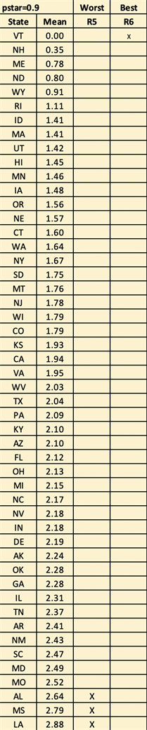
For k = 50, n = 8, and P^* = 0.90, the constants d = c = 1.2905σ. The value of σ is chosen to be 0.261 based on the two-way additive ANOVA of the transformed SHRs (i.e., the square root of the Mean Square for Error) as shown in Table 3.

Figure 1. Residual plots for SHR^0.4 from a two-way additive ANOVA. (a) Distribution of transformed data; (b) Residual probability plot.

Table 3. Two-way ANOVA table for the transformed SHRs.

Both the factors state and year are shown to be highly significant in affecting the variability of the transformed SHRs, i.e., their p-values are approximately zero.

Then d = c = 1.2905 × 0.261 = 0.34. The means of the transformed rates are given in Appendix C. The maximum sample mean is 2.88 (LA) and the minimum sample mean is 0.00 (VT).

For selecting the “worst” subset,

R₅: Select the ith state iff ${\bar{X}}_i\ge {\bar{X}}_{\left[k\right]}-d=2.88-0.34=2.54$.

The three states AL, MS, LA are chosen.

For selecting the “best” subset,

R₆: Select the ith state iff ${\bar{X}}_i\le {\bar{X}}_{\left[1\right]}+c=0.00+0.34=0.34$.

Only the state of VT is chosen for the selected subset.

An advantage of the parametric approach over the nonparametric approach is that the parametric analysis explicitly utilizes the magnitudes of the data rather than simply their rank values. Thus, in this analysis, the normal means parametric approach results in a dramatic reduction in the number of states chosen for the selected subsets. These results are displayed in Figure 2.

5. Bayesian Approach to the Selection Problem

In this section, a Bayesian approach is adopted and the population means are assumed to be stochastic. The idea is quite straightforward. A posterior distribution on the population means is used to simulate a large number of random draws, or realizations, of those means. With those draws, ordering probabilities of the population means can be estimated. And from these estimates, simple calculations can provide estimates of, e.g., the probability that a specific population

Figure 2. Selected states using parametric rules.

mean is greater than all the other population means. There are many choices that can be made for the posterior distributions. One such approach, utilizing flat (or noninformative) prior distributions on the population means is illustrated here.

As shown in Gill [10] and many other Bayesian texts, the posterior distribution of the mean of the ith population (state), μ_i, is normal with mean ${\bar{X}}_i$ and standard deviation $\sigma /\sqrt{n}$, i = 1, ∙∙∙, k. In this situation, the Bayesian and frequentist results (via Central Limit Theorem) are very similar in form. The relevant calculations become

$P\left({\mu }_{m_1}\le {\mu }_{m_2}\le \cdots \le {\mu }_{m_k}\right)$, (10)

where (m₁, m₂, ∙∙∙, m_k) is any of the k factorial permutations of the integers (1, 2, ∙∙∙, k). For example, for k = 4, there would be 4! = 24 such probabilities to calculate. This can be easily handled with WinBugs (an MCMC simulator) or R. For frequentists, these calculations are meaningless. This approach is used in both of the following subsections. In section “Example with k = 4”, all of the permutation probabilities (10) can be estimated with simulated draws of the posterior mean as k is small. In section “Bayesian Analysis of SHR^0.4” using R, with large k, applicable to the analysis of SHR^0.4, a convenient function in R is used to identify which population (state) realizes the largest and smallest posterior mean on each simulation pass.

5.1. Example with k = 4

Suppose we have k = 4 populations with three observations from each of the populations yielding sample means of 2, 3, 4, and 5. Assume a common known standard deviation equal to 1 and a flat (noninformative) prior distribution on the population means. Using, for example, WinBugs, all 24 values of the probabilities given in Equation (10) can be computed. By appropriate summing, the estimated values of P[μ_i = max(μ_j)], i = 1, 2, 3, 4, are obtained. Table 4 gives the results of such computations for 6 of the 24 parameter permutations. These are the 6 permutations, where μ₄ is the largest of the four means.

The tabled values were generated with WinBugs using the model code given in Appendix D and specifying a large number (10⁵) draws on the posterior means. The probabilities of the permutations, $P\left({\mu }_{m_1}\le {\mu }_{m_2}\le {\mu }_{m_3}\le {\mu }_{m_4}\right)$, are denoted by P1.2.3.4 in Table 4.

Given the probabilities in Table 4, it now follows that P(μ₄ is max) = 0.6844 + 0.1031 + ∙∙∙ + 0.0012 = 0.8873, i.e., the sum of the six probabilities in the Table. In a similar manner, the calculations yielded P(μ₁ is max) = 0.00006, P(μ₂ is max) = 0.00364, and P(μ₃ is max) = 0.10900. A complete probability distribution over all possible ordering of the population means is realized. This approach of calculating all the permutation probabilities is, from a practical vantage, limited to small values of k (say k≤ 5 or 6). In our application to homicide rates where k = 50, another Bayesian approach is more useful as described in the next subsection.

Table 4. A sampling of WinBugs estimates for selection from four populations.

Figure 3. Selected states using Bayesian rules.

5.2. Bayesian Analysis of SHR^0.4 Using R

The power transformation makes plausible the negligible interaction assumption for the additive model. The “state effects”, assuming flat normal priors, have a normal distribution centered at ${\bar{X}}_i$ and standard deviation $\sigma /\sqrt{n}$, i = 1, ∙∙∙, k. We now simulate in R a draw from each state, rank the results (using “which.max” and “which.min”), and repeat a large number of times (e.g., 10⁶) to obtain P(LA is worst) = 0.74702, P(MS is worst) = 0.20606, P(AL is worst) = 0.04209, P(VT is best) = 0.99768. These results are displayed in Figure 3. The R code for these calculations is given in Appendix E.

The results of the Bayesian analysis herein presented are in close agreement with the results given by the parametric selection procedure. This is as expected since the choice of a noninformative prior distribution results in an analysis based on the likelihood function as is the parametric selection procedure.

6. Concluding Remarks

The subset selection procedures, parametric or nonparametric, select a random number of populations to include in the subsets on which a confidence statement can be attached. Subset size is a random variable dependent on the observed data. Determining the constants required to implement the selection rules does require the determination of the Least Favorable Configuration (LFC), i.e., the configuration of population parameters minimize the probability of a CS. With two of the procedures used in this article, R₁ and R₃, that determination has been made only in the situation where the underlying parameter space is a “slippage” space, i.e., all population parameters are equal with the possible exception of one.

The nonparametric selection rules choose a much larger subset than the parametric procedures. And the conclusions from the Bayesian analyses are qualitatively closely aligned with those from the parametric selection procedures. This is not surprising as the nonparametric approach uses the ranks of the data, not the magnitudes. And as seen in Figure 1, there are outliers on the lower and upper end of the residual probability plot.

Bayesian procedures can yield a complete probability distribution over all orderings of the population parameters (e.g., means). There is a curse of dimensionality—k! gets large very quickly. However, using simulation capability in WinBugs and R, it is straightforward to generate a probability distribution over the populations as to which has the maximum (minimum) parameter. This was illustrated with SHRs from k = 50 states.

The SHR results have been compared to MVTFRs conducted by McDonald [11]. The “worst” states selected for SHR are AL, MS, and LA while SC, MT, and MS for MVTFR. The “best” states selected for SHR is VT while MA for MVTFR. This is some consistency since the “worst” states are mostly from the Southeastern states and the “best” states are both from the Northeast.

Appendix A. State Homicide Rates Raised to 0.4 Power

State 2005 2014 2015 2016 2017 2018 2019 2020

AK 1.93 1.86 2.30 2.21 2.57 2.24 2.59 2.21

AL 2.47 2.31 2.53 2.68 2.78 2.72 2.77 2.89

AR 2.30 2.26 2.23 2.38 2.49 2.42 2.45 2.79

AZ 2.41 1.90 1.98 2.09 2.13 2.06 2.03 2.24

CA 2.17 1.84 1.90 1.95 1.92 1.87 1.83 2.06

CO 1.71 1.61 1.69 1.79 1.84 1.86 1.79 2.02

CT 1.59 1.53 1.67 1.49 1.59 1.51 1.57 1.84

DE 2.13 2.13 2.24 2.18 2.17 2.15 2.06 2.50

FL 2.02 2.07 2.09 2.15 2.10 2.13 2.14 2.27

GA 2.19 2.13 2.21 2.29 2.29 2.26 2.31 2.56

HI 1.29 1.37 1.37 1.51 1.44 1.57 1.44 1.61

IA 1.21 1.44 1.44 1.51 1.63 1.49 1.49 1.67

ID 1.59 1.42 1.32 1.29 1.55 1.40 1.24 1.44

IL 2.15 2.07 2.17 2.43 2.41 2.30 2.31 2.63

IN 2.03 2.01 2.05 2.25 2.20 2.23 2.20 1.48

KS 1.72 1.67 1.86 1.95 2.11 2.03 1.89 2.18

KY 1.96 1.86 2.02 2.20 2.21 2.06 2.03 2.46

LA 2.77 2.67 2.74 2.90 2.91 2.82 2.93 3.31

MA 1.51 1.32 1.35 1.35 1.47 1.40 1.40 1.49

MD 2.55 2.14 2.54 2.52 2.53 2.44 2.51 2.65

ME 1.24 1.32 1.24 0.00 0.00 0.00 1.27 1.21

MI 2.17 2.09 2.10 2.14 2.09 2.11 2.11 2.38

MN 1.49 1.29 1.51 1.42 1.37 1.40 1.51 1.67

MO 2.21 2.24 2.47 2.50 2.64 2.65 2.59 2.87

MS 2.41 2.65 2.64 2.71 2.76 2.82 2.99 3.35

MT 1.63 1.53 1.74 1.79 1.79 1.78 1.69 2.13

NC 2.25 1.99 2.06 2.23 2.17 2.10 2.18 2.36

ND 0.00 0.00 1.57 0.00 0.00 1.44 1.57 1.81

NE 1.44 1.63 1.74 1.61 1.49 1.29 1.57 1.76

NH 0.00 0.00 0.00 0.00 0.00 1.27 1.51 0.00

NJ 1.92 1.81 1.83 1.84 1.76 1.69 1.63 1.79

NM 2.29 2.15 2.30 2.45 2.35 2.59 2.68 2.59

NV 2.27 2.09 2.14 2.23 2.25 2.26 1.98 2.21

NY 1.86 1.63 1.63 1.67 1.55 1.59 1.59 1.86

OH 1.99 1.93 2.05 2.11 2.24 2.15 2.13 2.42

OK 2.06 2.13 2.35 2.36 2.35 2.18 2.39 2.41

OR 1.53 1.42 1.63 1.61 1.57 1.44 1.55 1.71

PA 2.09 1.93 1.99 2.05 2.13 2.10 2.06 2.35

RI 1.57 1.44 1.51 1.40 0.00 0.00 1.44 1.55

SC 2.29 2.25 2.46 2.41 2.44 2.53 2.61 2.76

SD 1.53 1.57 1.78 1.86 1.78 1.72 1.67 2.11

TN 2.33 2.11 2.20 2.39 2.39 2.43 2.43 2.66

TX 2.11 1.93 1.99 2.05 2.02 1.96 2.03 2.25

UT 1.42 1.32 1.32 1.44 1.47 1.37 1.47 1.53

VA 2.10 1.76 1.83 1.98 1.96 1.92 1.95 2.10

VT 0.00 0.00 0.00 0.00 0.00 0.00 0.00 0.00

WA 1.67 1.57 1.63 1.53 1.67 1.69 1.59 1.78

WI 1.79 1.55 1.83 1.87 1.69 1.72 1.78 2.06

WV 1.96 2.03 1.83 2.09 2.11 2.02 2.01 2.18

WY 0.00 1.81 0.00 0.00 0.00 1.76 1.81 1.89

Appendix B. State Rank Sums and Subsets of States Chosen by Nonparametric Rules

Appendix C. Ordered Means of State SHR^0.4

Appendix D. WinBugs Code for Calculations Related to Table 4

# Ranking & Selection for k = 4 populations

model {

for (i in 1:3) {

x1[i] ~ dnorm(m1,tau1)

x2[i] ~ dnorm(m2,tau2)

x3[i] ~ dnorm(m3,tau3)

x4[i] ~ dnorm(m4,tau4)

}

m1 ~ dnorm(a,b)

m2 ~ dnorm(a,b)

m3 ~ dnorm(a,b)

m4 ~ dnorm(a,b)

tau1 <- pow(sigma1,-2)

tau2 <- pow(sigma2,-2)

tau3 <- pow(sigma3,-2)

tau4 <- pow(sigma4,-2)

p1.2.3.4 <- step(m2-m1)*step(m3-m2)*step(m4-m3)

p1.2.4.3 <- step(m2-m1)*step(m4-m2)*step(m3-m4)

p1.3.2.4 <- step(m3-m1)*step(m2-m3)*step(m4-m2)

p1.3.4.2 <- step(m3-m1)*step(m4-m3)*step(m2-m4)

p1.4.2.3 <- step(m4-m1)*step(m2-m4)*step(m3-m2)

p1.4.3.2 <- step(m4-m1)*step(m3-m4)*step(m2-m3)

p2.1.3.4 <- step(m1-m2)*step(m3-m1)*step(m4-m3)

p2.1.4.3 <- step(m1-m2)*step(m4-m1)*step(m3-m4)

p2.3.1.4 <- step(m3-m2)*step(m1-m3)*step(m4-m1)

p2.3.4.1 <- step(m3-m2)*step(m4-m3)*step(m1-m4)

p2.4.1.3 <- step(m4-m2)*step(m1-m4)*step(m3-m1)

p2.4.3.1 <- step(m4-m2)*step(m3-m4)*step(m1-m3)

p3.1.2.4 <- step(m1-m3)*step(m2-m1)*step(m4-m2)

p3.1.4.2 <- step(m1-m3)*step(m4-m1)*step(m2-m4)

p3.2.1.4 <- step(m2-m3)*step(m1-m2)*step(m4-m1)

p3.2.4.1 <- step(m2-m3)*step(m4-m2)*step(m1-m4)

p3.4.1.2 <- step(m4-m3)*step(m1-m4)*step(m2-m1)

p3.4.2.1 <- step(m4-m3)*step(m2-m4)*step(m1-m2)

p4.1.2.3 <- step(m1-m4)*step(m2-m1)*step(m3-m2)

p4.1.3.2 <- step(m1-m4)*step(m3-m1)*step(m2-m3)

p4.2.1.3 <- step(m2-m4)*step(m1-m2)*step(m3-m1)

p4.2.3.1 <- step(m2-m4)*step(m3-m2)*step(m1-m3)

p4.3.1.2 <- step(m3-m4)*step(m1-m3)*step(m2-m1)

p4.3.2.1 <- step(m3-m4)*step(m2-m3)*step(m1-m2)

p[1] <- p1.2.3.4

p[2] <- p1.2.4.3

p[3] <- p1.3.2.4

p[4] <- p1.3.4.2

p[5] <- p1.4.2.3

p[6] <- p1.4.3.2

p[7] <- p2.1.3.4

p[8] <- p2.1.4.3

p[9] <- p2.3.1.4

p[10]<- p2.3.4.1

p[11]<- p2.4.1.3

p[12]<- p2.4.3.1

p[13]<- p3.1.2.4

p[14]<- p3.1.4.2

p[15]<- p3.2.1.4

p[16]<- p3.2.4.1

p[17]<- p3.4.1.2

p[18]<- p3.4.2.1

p[19]<- p4.1.2.3

p[20]<- p4.1.3.2

p[21]<- p4.2.1.3

p[22]<- p4.2.3.1

p[23]<- p4.3.1.2

p[24]<- p4.3.2.1

p.sum <- sum(p[])

}

list(a=0,b=0.001,x1=c(1,2,3),x2=c(2,3,4),x3=c(3,4,5),x4=c(4,5,6),

sigma1=1,sigma2=1,sigma3=1,sigma4=1)

Appendix E. R Code for Bayesian Simulations Described in the Bayesian Analysis of SHR^0.4 Section

# R-code for Bayesian simulations of Rate^0.4

# k = number of populations; n = number of simulations

# sigma = model sd ; m = number of years

k=50; n=100000; sigma=0.261; m=8

# sigma value is estimate from two-way ANOVA of Rate^0.4

# mu values are means of (Rate^0.4)

x <- c(rep(0,k))

y <- c(rep(0,n))

z <- c(rep(0,n))

err <- sigma/sqrt(m)

mu <- c(2.24, 2.64, 2.41, 2.10, 1.94, 1.79, 1.60, 2.19, 2.12, 2.28, 1.45, 1.48,

1.41, 2.31, 2.18, 1.93, 2.10, 2.88, 1.41, 2.49, 0.78, 2.15, 1.46, 2.52, 2.79,

1.76, 2.17, 0.80, 1.57, 0.35, 1.78, 2.43, 2.18, 1.67, 2.13, 2.28, 1.56, 2.09,

1.11, 2.47, 1.75, 2.37, 2.04, 1.42, 1.95, 0.00, 1.64, 1.79, 2.03, 0.91)

names(mu) <- c("AK","AL","AR","AZ","CA","CO","CT","DE",

"FL","GA","HI","IA","ID","IL","IN","KS",

"KY","LA","MA","MD","ME","MI","MN","MO",

"MS","MT","NC","ND","NE","NH","NJ","NM",

"NV","NY","OH","OK","OR","PA","RI","SC",

"SD","TN","TX","UT","VA","VT","WA","WI",

"WV","WY")

mu

for (i in 1:n){

for (j in 1:k) {x[j] <- rnorm(1, mean = mu[j], sd = err)}

y[i] <- which.min(x)

z[i] <- which.max(x)

}

table(y)

table(z)

Conflicts of Interest

The authors declare no conflicts of interest regarding the publication of this paper.

References

[1]	Elinson, Z. (2021) U.S. Murders Up Nearly 30% in 2020, FBI Says. Wall Street Journal, September 28, page A3.
[2]	Green, J. and McDonald, G.C. (2009) Nonparametric Subset Selection Procedures: Applications and Properties. American Journal of Mathematical and Management Sciences, 29, 413-436. https://doi.org/10.1080/01966324.2009.10737766
[3]	McDonald, G.C. (1979) Nonparametric Selection Procedures Applied to State Traffic Fatality Rates. Technometrics, 21, 515-523. https://doi.org/10.1080/00401706.1979.10489822
[4]	McDonald, G.C. (1972) Some Multiple Comparison Selection Procedures Based on Ranks. Sankhyā: The Indian Journal of Statistics, Series A, 34, 53-64.
[5]	McDonald, G.C. (1973) The Distribution of Some Rank Statistics with Applications in Block Design Selection Problems. Sankhyā: The Indian Journal of Statistics, Series A, 35, 187-204.
[6]	McDonald, G.C. (1985) Characteristics of Block Design Selection Procedures and A Counterexample. Sankhyā: The Indian Journal of Statistics, Series A, 47, 47-55.
[7]	Gupta, S.S., Nagel, K. and Panchapakesan, S. (1973) On the Order Statistics from Equally Correlated Normal Random Variables. Biometrika, 60, 403-413. https://doi.org/10.1093/biomet/60.2.403
[8]	McDonald, G.C. (2021) Computing Probabilities for Rank Statistics Used with Block Design Nonparametric Subset Selection Rules. American Journal of Mathematical and Management Sciences, 41, 38-50. https://doi.org/10.1080/01966324.2021.1910885
[9]	Gupta, S.S. (1965) On Some Multiple Decision (Ranking and Selection) Rules. Technometrics, 7, 225-245. https://doi.org/10.1080/00401706.1965.10490251
[10]	Gill, J. (2015) Bayesian Methods: A Social and Behavioral Sciences Approach. 3rd Edition. Taylor & Francis Group, Boca Raton.
[11]	McDonald, G.C. (2016) Applications of Subset Selection Procedures and Bayesian Ranking Methods in Analysis of Traffic Fatality Rates. WIREs Computational Statistics, 8, 222-237. https://doi.org/10.1002/wics.1385