Food and Nutrition Sciences, 2013, 4, 252-261
http://dx.doi.org/10.4236/fns.2013.43034 Published Online March 2013 (http://www.scirp.org/journal/fns)
An Application of Wavelet Analysis to Meat Consumption
Cycles
Marija Banović1,2,3*, Luis Catela Nunes2, Vladan Arsenijevic4
1CIISA—Faculty of Veterinary Medicine, Technical University of Lisbon, Lisbon, Portugal; 2INOVA—Nova School of Business
and Economics, Nova University of Lisbon, Lisbon, Portugal; 3MAPP—Aarhus School of Business, Aarhus University, Aarhus,
Denmark; 4SIM—Faculty of Sciences, University of Lisbon, Lisbon, Portugal.
Received January 22nd, 2013; revised February 22nd, 2013; accepted March 4th, 2013
ABSTRACT
The existence or nonexistence of changes in meat consumption cycles is critical to meat industry. If the change is exis-
tent, there is a need to understand what motivates the change to identify the most appropriate response. Wavelet analy-
sis is considered here as a promising technique that may lead to a better understanding of characteristic patterns and
changes in the meat consumption cycles.
Keywords: Meat Consumption Cycles; Wavelet Analysis
1. Introduction
Changes in the meat consumption cycles have been the
focus of much research over the last decades [1-4]. Even
though considerable effort has been put through on stud-
ies examining the demand for meats the debate is still
going around the factors causing these changes [5-8].
Whatever the explanation may be, the existence or
nonexistence of changes in meat consumption cycles is
of paramount importance for the meat industry in order
to remain competitive in the market. If the change is ex-
istent, there is a need to understand what motivates this
change in order to identify the most appropriate response.
Accordingly, if the explanation behind the change is that
consumer preferences have altered and white meat is
preferred, industry needs to take action and allocate re-
sources to research, product development and advertising.
If the change is nonexistent and changes in meat con-
sumption cycles can be explained by alterations in rela-
tive prices then the red meat industry should devote all
efforts to produce alternatives that will be able to com-
pete with the white meats on price. Determining whether
the changes in the meat consumption cycles have oc-
curred, what motivated them, their duration, and if they
repeat over time, is critical for the future industry poli-
cies. Inability to detect their occurrence or nonoccurrence
could come out costly for the meat industry.
Wavelet analysis has already been successfully applied
in a wide variety of disciplines, such as economics, fi-
nance, physics, and engineering [9-13]. This proficient
approach has also been used in agriculture and food
quality inspection where it can very well resolve issues
of signal processing in various systems used for quality
assessment of food products [14]. For example, wavelet
analysis has been used to characterize the surface texture
of fresh meat giving the predictive models of meat pal-
atability [15].
The typical approach in meat demand studies has been
to employ different techniques using only time-domain,
giving quite mixed results and complicating any defini-
tive conclusion about the existence or nonexistence of
changes in the meat consumption cycles. However, im-
portant relations also exist in the frequency domain which
cannot be adequately studied using the standard methods.
For example, it is possible that consumers react to news
about BSE outbreak in the short-run, while in the long-
run, the consumption levels are essentially determined by
their income. Or, it is possible that the effects of a certain
policy may change and evolve over time, therefore af-
fecting the consumption cycles in different ways at dif-
ferent frequencies. The ability to explain the nature and
detect dominant patterns in the meat consumption cycles
may be one of the most important ways to understand
changes in the meat sector, as it also affects other food
sectors, both upstream and downstream. Understanding
the patterns in the meat consumption cycles may also
assist in designing policies affecting the industry and
economies where meat production and processing are
important economic activities.
*Corresponding author.

An Application of Wavelet Analysis to Meat Consumption Cycles 253
Using the wavelet analysis, this research provides a
basis for the identification of characteristic patterns or
structures in the meat consumption cycles, which are
often masked in the traditional methods. Furthermore, it
checks if these patterns exist in other factors (e.g., prices,
income), often related to the changes in the meat con-
sumption cycles, and if such relations have evolved over
time. For this purpose, several tools are utilized: the
wavelet power spectrum, the cross-wavelet spectrum, the
wavelet coherence, and the wavelet phase. These tech-
niques show how the use of wavelet analysis may help to
unravel time-frequency relationships that would other-
wise remain hidden.
This study proceeds as follows. In Section 2, we de-
scribe and discuss the wavelet analysis, continuous wave-
let transform, wavelet tools, as well as the advantages of
wavelet over Fourier transform. Section 3 presents the
results of applying wavelet tools to meat consumption
cycles and discuss its insights. Section 4 concludes.
2. Wavelet Analysis
The wavelet transform is a powerful tool for analyzing
economic time-series data characterized by nonlinear dy-
namics. It allows for a variable-size view of the eco-
nomic time-series data studying at the same time its time
and frequency properties. Thus, the wavelet analysis en-
ables the researcher to separate out a time-series into its
constituent multiresolution components [9]. In this way
very fine details are detected in a time-series, as well as
particular characteristics, patterns, changes, discontinui-
ties and self-similarity that are often some of the most
interesting features of a time-series. Furthermore, differ-
ent relationships between economic variables that can
possibly be found at the disaggregate level rather than at
an aggregate level may be analyzed. This section intends
to provide some intuition and the necessary knowledge
for the discussion of the empirical results. For more de-
tails about wavelet technique [13,16-18].
2.1. Continuous Wavelet Transform
Wavelet analysis examines a time-series by cutting it into
small waves of different frequency which are localized in
time. In particular, wavelets are obtained by shifting and
scaling a specific function ψ(t), called the mother wavelet,
and are defined as:

,
1
s
t
t
s
s









(1)
where the parameter τ determines the wavelet localiza-
tion in time, and the parameter s determines the scale or
width of the wavelet. A low value of the scale parameter
s results in a high frequency wavelet capable of capturing
localized short cycles, and vice versa. The large scales
(or in terms of frequencies, the low frequencies) corre-
spond to overall information of a time-series, while small
scales (high frequencies) correspond to a detailed view.
Thus, high frequencies are used to isolate very fine de-
tails in a time-series (i.e., changes that occur in a short-
run), while the low frequencies can identify coarse de-
tails (i.e., changes that occur in a long-run).
The mother wavelet ψ(t) is simply an oscillating func-
tion of time that first grows and then decays and obeys
two conditions. The first condition is that the function ψ(t)
has a zero mean in the time domain:

d0tt 

 
. (2)
The second condition consists of a normalization re-
quirement:

2d1tt


 
, (3)
and is also known as the unit energy condition. The most
commonly used mother wavelet function is the Mo rle t
wavelet given by

2
0
1
M4
π,
t
it
tee



2
,
s
(4)
where i is the imaginary number and ω0 is the central
frequency of the wavelet. In order to study time-varying
frequency features, the Morlet wavelet with ω0 = 6 is an
optimal choice, as it gives the best balance between time
and frequency domains [11,17]. The choice of the mother
wavelet will depend on the features of a time-series that
will be decomposed. Depending on the application, mother
wavelet should be as similar as possible to a time-series
(or to its portion under analysis). In our case, and after
series of tests with different bases, the Morlet wavelet is
found to be the optimal option (choice). The continuous
wavelet transform (CWT) of a time-series x(t) with re-
spect to ψ(t) is given by the convolution:
 
,
,d
x
Wsxt tt




 (5)
where the asterisk * denotes the complex conjugate. As
with the Fourier counterpart, it is possible to recover the
original time-series from the wavelets by using an in-
verse wavelet transform that integrates over all the time
and frequency space.
The CWT of a time-series defined in discrete time


1, ,
t
x
tN
s
, assuming a uniform unit time step, is
obtained as:
 
,
1
,
N
xt
t
Wsx t




. (6)
Computation of the CWT is usually undertaken over
the whole time dimension τ and over a range of relevant
scales s. In this manner a fairly good approximation of a
given time-series is obtained by using only a few dozen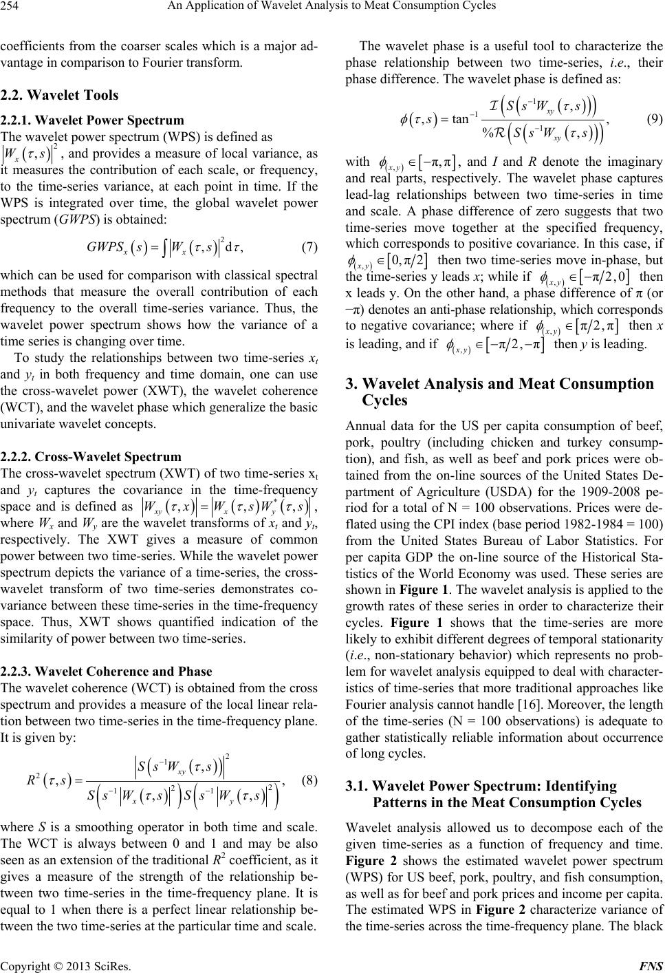

An Application of Wavelet Analysis to Meat Consumption Cycles 254
coefficients from the coarser scales which is a major ad-
vantage in comparison to Fourier transform.
2.2. Wavelet Tools
2.2.1. Wavelet Power Spectrum
The wavelet power spectrum (WPS) is defined as

2
,
x
Ws  , and provides a measure of local variance, as
it measures the contribution of each scale, or frequency,
to the time-series variance, at each point in time. If the
WPS is integrated over time, the global wavelet power
spectrum (GWPS) is obtained:
 
2
,d
xx
GWPS sWs,

  (7)
which can be used for comparison with classical spectral
methods that measure the overall contribution of each
frequency to the overall time-series variance. Thus, the
wavelet power spectrum shows how the variance of a
time series is changing over time.
To study the relationships between two time-series xt
and yt in both frequency and time domain, one can use
the cross-wavelet power (XWT), the wavelet coherence
(WCT), and the wavelet phase which generalize the basic
univariate wavelet concepts.
2.2.2. Cross-Wavelet Spectrum
The cross-wavelet spectrum (XWT) of two time-series xt
and yt captures the covariance in the time-frequency
space and is defined as




*
,,
xyx y
WxWsWs  ,  ,
where Wx and Wy are the wavelet transforms of xt and yt,
respectively. The XWT gives a measure of common
power between two time-series. While the wavelet power
spectrum depicts the variance of a time-series, the cross-
wavelet transform of two time-series demonstrates co-
variance between these time-series in the time-frequency
space. Thus, XWT shows quantified indication of the
similarity of power between two time-series.
2.2.3. Wavelet Coherence and Phase
The wavelet coherence (WCT) is obtained from the cross
spectrum and provides a measure of the local linear rela-
tion between two time-series in the time-frequency plane.
It is given by:
 





2
1
2
2 2
11
,
,
,,
xy
xy
SsW s
Rs
Ss WsSsWs





, (8)
where S is a smoothing operator in both time and scale.
The WCT is always between 0 and 1 and may be also
seen as an extension of the traditional R2 coefficient, as it
gives a measure of the strength of the relationship be-
tween two time-series in the time-frequency plane. It is
equal to 1 when there is a perfect linear relationship be-
tween the two time-series at the particular time and scale.
The wavelet phase is a useful tool to characterize the
phase relationship between two time-series, i.e., their
phase difference. The wavelet phase is defined as:
 
 

 
1
1
1
,
,tan
%,
xy
xy
SsW s
s
SsW s

 






,
(9)
with



,π,π xy
  , and I and R denote the imaginary
and real parts, respectively. The wavelet phase captures
lead-lag relationships between two time-series in time
and scale. A phase difference of zero suggests that two
time-series move together at the specified frequency,
which corresponds to positive covariance. In this case, if



, then two time-series move in-phase, but
the time-series y leads x; while if

0, π2
xy
 


,xy then
x leads y. On the other hand, a phase difference of π (or
−π) denotes an anti-phase relationship, which corresponds
to negative covariance; where if
π2,0  



,π2,π xy
  then x
is leading, and if



,π2, π xy


 then y is leading.
3. Wavelet Analysis and Meat Consumption
Cycles
Annual data for the US per capita consumption of beef,
pork, poultry (including chicken and turkey consump-
tion), and fish, as well as beef and pork prices were ob-
tained from the on-line sources of the United States De-
partment of Agriculture (USDA) for the 1909-2008 pe-
riod for a total of N = 100 observations. Prices were de-
flated using the CPI index (base period 1982-1984 = 100)
from the United States Bureau of Labor Statistics. For
per capita GDP the on-line source of the Historical Sta-
tistics of the World Economy was used. These series are
shown in Figure 1. The wavelet analysis is applied to the
growth rates of these series in order to characterize their
cycles. Figure 1 shows that the time-series are more
likely to exhibit different degrees of temporal stationarity
(i.e., non-stationary behavior) which represents no prob-
lem for wavelet analysis equipped to deal with character-
istics of time-series that more traditional approaches like
Fourier analysis cannot handle [16]. Moreover, the length
of the time-series (N = 100 observations) is adequate to
gather statistically reliable information about occurrence
of long cycles.
3.1. Wavelet Power Spectrum: Identifying
Patterns in the Meat Consumption Cycles
Wavelet analysis allowed us to decompose each of the
given time-series as a function of frequency and time.
Figure 2 shows the estimated wavelet power spectrum
(WPS) for US beef, pork, poultry, and fish consumption,
as well as for beef and pork prices and income per capita.
The estimated WPS in Figure 2 characterize variance of
the time-series across the time-frequency plane. The black

An Application of Wavelet Analysis to Meat Consumption Cycles 255
Figure 1. Time-series.
contour designates the 5% significance level. The regions
with high variance (or high power) are presented by red
color, while the regions with low variance (or low power)
are depicted by blue color.
Figure 2 points to some characteristic patterns of the
time-series. The common characteristic of the analyzed
time-series is that they exhibit a greater volatility until
the late 1950s, which is reflected by higher WPS (i.e., the
variance of the time-series). This is quite unlike the sec-
ond half of the century where volatility decreases, point-
ing to the beginning of the 1960s as a significant step in
time when a structural change occurred.
The analysis of the WPS further reveals two types of
common cycles across meats: short ones with a periodic-
ity of 2 - 4 years, which characterize beef, pork, and
poultry consumption; and longer cycles with a periodic-
ity of around 8 years for the beef and poultry consump-
tion. Especially interesting are the short cycles during the
first half of the century when the time-series are charac-
terized by greater volatility. On the other hand, the longer
cycles of beef and poultry disappear after the 1950s.
An important finding is that the pork consumption be-
haves in a rather unique manner when compared to the
other meats. Pork consumption exhibits no evidence of
long cycles, only short cycles with 2 - 4-year periodicity
during the 1970s. Two types of mechanism are responsi-
ble for this distinct behavior of pork consumption. First,
the more stable and repetitive short cycles in pork con-
sumption point to the insensitivity of pork consumption
to changes in own prices and incomes (see next two sub-
sections). Second, the fact that short cycles continue
throughout the 1970s is particularly interesting, and this
is probably influenced by changes in production practices
in the US pork industry during the 1970s. In that decade
the US pork industry improved breeding and husbandry
practices and began trimming outside fat on retail cuts,
which lowered the fat content of pork [8]. This might
have led consumers to perceive pork as healthier (con-
taining less fat, calories and cholesterol) reflecting more
stability in pork consumption.
The estimated WPS of beef and pork prices differ. The
pork prices display shorter cycles with 2 - 6 years perio-
dicity until the 1950s, while beef prices show rather long
cycles with 2 - 10-year periodicity around the 1940s. In-
come has a major peak close to the 8 year periodicity,
coinciding with the long cycles and a minor peak at the 2
- 4-year band corresponding to the shorter cycles in meat
consumption found earlier. These cycles correspond to
the business cycle frequencies reported in the literature
(see e.g. [10]). As seen from Figures 2(e)-(g) these cy-
cles appear only up to the mid 1950s, which is in line
with the Great Moderation period found for the US
economy after this time.
3.2. Cross-Wavelet Spectrum: Understanding
Common Features in the Meat Consumption
Cycles
The cross-wavelet power spectrum (XWT) estimate shows
the common features of any two time-series. Figure 3
demonstrates the pattern similarity in the time-series. The
black contour designates the 5% significance level. The
power similarity between two time-series is depicted by
color system ranging from blue-low covariance to red-
high covariance. The relative phase relationship is shown
as arrows with in-phase (positive covariance) pointing
right, and anti-phase (negative covariance) pointing left.
The results from Figure 3 confirm that there is a sig-
nificant covariance between the different time-series at
the shorter and longer cycles identified during the first
half of the century. In particular, the XWT of beef and
poultry consumption suggests a large interdependence
between these two time-series at 2 - 4-year cycles from
the early 1920s until the late 1950s, as well as in the 6 -
12-year cycles from the early 1930s until the late 1950s.
However, the XWT of pork and poultry consumption
exhibits highly significant areas of interdependence from
the 1920s to the late 1970s. Interestingly, poultry and fish
consumption show a large area of common power but in

An Application of Wavelet Analysis to Meat Consumption Cycles 256
Figure 2. Estimated wavelet power spectra (WPS) of time-series growth rates. The x-axis represents time in years, while the
y-axis shows period in years. The black contour designates the 5% significance level. The regions with high variance (or high
power) are presented by red color, while the regions with low variance (or low power) are depicted by blue color.
the 2 - 16-year band during the late 1920s until the 1960s.
Pork and fish consumption exhibit quite a similar pattern.
Figure 3(j) presents the relationship between income
and different types of meat and fish consumption where
the late 1950s and the beginning of 1960s has again been
confirmed as a turning-point in meat consumption time-
series, when significant changes occurred. The estimated
XWT shows higher sensitivity of meat consumption to
income changes until the late 1950s, shown by joint
power both at low and high scales. A similar pattern has
been observed for the relationship between beef con-
sumption and own prices. Nevertheless, the pork con-
sumption exhibits less sensitivity to own price, after the
late 1950s.
A similar pattern occurs in the association between
income and fish consumption. Since the relationship be-
tween income and meat consumption, as well as income
and fish consumption, is mainly in positive covariance
across all scales, it can be confirmed increased sensitivity
of meat and fish consumption to changes in income. This
is also evident even outside the cone of influence, point-
ing to important links between income and meat con-
sumption even after the decade of 2000s.
Since the XWT exposes regions with common features
(high common power) between two time-series, but does
not explain their local cross-correlation, i.e., their strength
of relationship, we further analyze wavelet coherence
and phase.
3.3. Wavelet Coherence and Phase: Unraveling
Strength of Factors Influencing the Meat
Consumption Cycles
The cross-wavelet coherence (WCT) checks for a sig-
nificant correlation between different time-series. Figure
4 displays the WCT estimates of the cross-correlation
between the different time-series as a function of cycle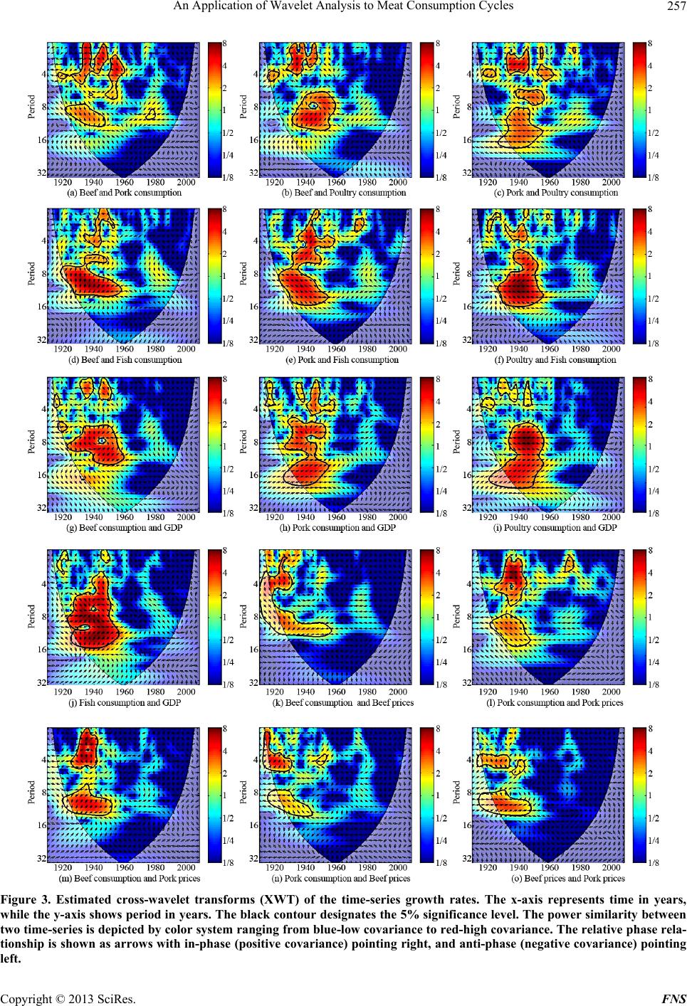

An Application of Wavelet Analysis to Meat Consumption Cycles 257
Figure 3. Estimated cross-wavelet transforms (XWT) of the time-series growth rates. The x-axis represents time in years,
while the y-axis shows period in years. The black contour designates the 5% significance level. The power similarity between
two time-series is depicted by color system ranging from blue-low covariance to red-high covariance. The relative phase rela-
tionship is shown as arrows with in-phase (positive covariance) pointing right, and anti-phase (negative covariance) pointing
left.

An Application of Wavelet Analysis to Meat Consumption Cycles 258
Figure 4. Estimated wavelet coherences (WCT) of time-series growth rates. The x-axis represents time in years, while the
y-axis shows period in years. The black contour designates the 5% significance level. The strength of relationship between
two time-series is explained by a color system ranging from blue-low coherency to red-high coherency. The mutual interac-
tion of time-series is shown by arrows. Arrows pointing to the right mean that the time-series are in-phase, while arrows
pointing to the left mean that the time-series are in anti-phase.

An Application of Wavelet Analysis to Meat Consumption Cycles 259
periodicity and time, showing their relationship strength
and mutual interaction. The black contour designates the
5% significance level. The strength of relationship be-
tween two time-series is explained by a color system
ranging from blue-low coherency to red-high coherency.
The mutual interaction (or locally phase locked behavior)
among time-series is shown by arrows. Arrows pointing
to the right mean that the time-series are in-phase, while
arrows pointing to the left mean that the time-series are
in anti-phase. When two time-series are in-phase arrows
pointing right and up mean that first time-series lags be-
hind second time-series, while to the right and down first
one leads second one. On the other hand, when two
time-series are in anti-phase arrows pointing left and up
show that first time-series leads second time-series, and
left and down indicate that first one lags behind second
one.
Figure 4 exposes several ranges of significant coher-
ence (dependence) between the different time-series. The
correlation between beef and poultry consumption is very
strong and significant from the beginning of the century
until the late 1950s in the 16 - 20-year band, during the
1980s in the 8 year band and in the 1990s around 3-year
band. For the longer periods and until the 1980s poultry
is led by beef, but in the 1990s poultry starts replacing
beef. This change in the way meat consumption is dis-
tributed across beef and poultry signalize the occurrence
of shifts in consumer preferences. This finding coincides
with the increased consumers’ awareness with health,
safety, and nutritional issues during the 1980s and 1990s,
when US consumers started to see beef as less desirable
than poultry in terms of fat, cholesterol, calorie content,
artificial ingredients, convenience characteristics, store
display, and price (too expensive) [2,4,19].
Figure 4(m) reveals a strong dependence of beef con-
sumption to changes in pork price, especially around 10-
year band. These time-series mutually interact in a way
that beef consumption is actually influenced by pork
prices. Moreover, Figure 4(n) demonstrates dependence
of beef prices to changes in pork consumption in the 8
year band, when pork consumption during the 1980s and
1990s leads beef prices. Figure 4(o) also shows that beef
and pork prices are highly interrelated and negatively
correlated.
A strong interrelationship between beef and fish con-
sumption is also observed in Figure 4(d), which is espe-
cially evident for the large cycle periodicity of 30 years.
It seems that fish in the long run might evolve from being
an unimportant commodity to a good that will be an im-
portant future protein opponent to meat. In fact, Wohl-
genant [19] pointed out that during the mid 1970s, the
relationship between beef and fish changed from one of
substitutability to one of complementarity. Nevertheless,
our results demonstrate that this relationship has been
prolonged to the end of 2000s.
The relationship between pork and poultry consump-
tion, Figure 4(c), is very synchronous (in-phase) around
the 16-year band and for all time periods, demonstrating
similar movement of their consumption cycles. The sec-
tors outside the cone of influence and above the 5% sig-
nificance level are not a reliable indicator of correlation,
however, the significant area of is so large that it is very
unlikely to be simply by chance, revealing again substi-
tution between these two meats. Figure 4(e) shows that
the coherence of pork and fish consumption is very sig-
nificant for a periodicity of 8 years at the beginning of
the century and until the 1950s, as well as in the 3 - 4-
year periodicity during the 1970s. These two series are
negatively correlated (in anti-phase), where fish con-
sumption lags behind pork consumption. However, the
behavior of these two time-series changes completely
during the late 1990s and 2000s, exhibiting a synchro-
nized pattern. This suggests that unlike the period until
the 1980s, when fish and pork consumption alternate, sub-
stituting one another, during the 1990s and 2000s they
tend to fluctuate in a similar manner. These are signifi-
cant results that again point to the exceptional behavior
of pork consumption cycles, which may be related to the
fact that in the 1990s pork contained more lean and less
fat due to the new production practices, in which the US
pork industry actually capitalized by promoting pork as a
light and nutritious alternative to poultry—“Pork: The
Other White Meat” [8]. Comparing the results for the
relationship between meat and fish consumption and in-
come (Figures 3 and 4), we see that the larger areas
stand out as being significant, showing a positive (in-
phase) relationship between the aforementioned time-
series, suggesting that meat and fish consumption ac-
company changes in income. The beef, pork, and poultry
consumption cycles with periodicities around 20 years
are strongly correlated with income cycles.
In Figure 4 the regions of higher coherence at lower to
medium scales may point to what is perhaps the most
interesting element of change regarding the relationship
between income and meat consumption (beef and poul-
try). While income and beef consumption, as well as in-
come and poultry consumption, show high mutual de-
pendence at medium to high scales and for most of the
period, the relationship between income and pork con-
sumption is more concentrated at higher scales. The in-
creased sensitivity of beef and poultry consumption to
changes in income, and decreased sensitivity of pork
consumption to income again points to uniqueness of
pork consumption cycles. The US pork industry has man-
aged to tackle the challenge of meeting the consumer
demands regarding pork that seems to be an entirely dif-
ferent product in the eyes of the consumers [8].
Unlike the association between income and meat con-

An Application of Wavelet Analysis to Meat Consumption Cycles 260
sumption, the relationship between income and fish con-
sumption accounts for much smaller regions of coher-
ence mostly at medium scales. This occurs during the
decade of the 1970s until the late 1980s, when the rela-
tionship between fish consumption and income displays a
strong cross-correlation that points to fish becoming an
important protein source at par with meat.
Our results show that meat consumption time-series
can significantly alter both in time and frequency and
that wavelet tools are good indicators of these alterations.
The finding that the beginning of 1960s represents an
important turning point in the evolution of US meat con-
sumption cycles, and that this significant structural change
was not completed until the decade of the 2000s, is a
rather important contribution to the research on meat
consumption cycles. Moreover, the wavelet analysis un-
dertaken here demonstrates not only changes of the meat
consumption cycles in time, but also in frequency. The
findings of the different meat consumption patterns is
also particularly interesting, especially pork consumption
cycles that exhibit more stability at the shorter cycles,
showing no evidence of long cycles, and thus pointing to
the fact that the pork consumption is less sensitive to
external shocks.
4. Conclusions
This paper has used wavelet analysis to understand char-
acteristic features, patterns and changes in the meat con-
sumption cycles for the United States data. The real-
world data, such as meat consumption time-series, often
have complex dynamics that dominate their behavior.
Wavelet analysis has the potential to deal with nonsta-
tionary data, while most econometric methods assume
stationarity, which may or may not be apparent in eco-
nomic data. Furthermore, wavelets ability to separate out
the dynamics in a time-series over a different time hori-
zons, can reveal interesting insights into cycles at differ-
ent time scales. Besides common analysis in the time
domain that can be done using other techniques, wavelet
analysis can also capture the hidden information on con-
sumption cycles in the frequency domain, where the
evolution of the wavelet transform from one scale to an-
other is easy to follow and reconstruct, isolating very fine
details or changes that occur in a short-run (using high
frequencies), and very large details or changes that occur
in a long-run (using low frequencies). By applying the
wavelet approach, we have shown its potential in exam-
ining meat consumption cycles, as well as interactions
between different time-series, representing them in a
time-frequency plane where features and patterns (we
could not otherwise see) can be observed in an analytical
way.
The US meat industry has been a major force in US
agriculture and is currently undergoing significant change.
In order to be able to respond to consumer demand and
adapt production patterns and practices it is important to
capture any systematic pattern that eventually occurs in
the meat consumption cycles, especially at coarse scales
which determine global trends, as they influence global
environment. Our analysis has demonstrated significant
structural change in meat consumption cycles initiated in
the 1960s and not completed until the decade of the
2000s, patterns of two types of prevailing cycles: longer
with 8-year periodicity and shorter with 2 - 4-year perio-
dicity characterized by greater volatility. Moreover, we
have shown that pork consumption exhibit more stability
at the shorter cycles, showing no evidence of long cycles.
Facing changes in the meat sector the identification and
understanding of the specificities of these global trends
could help the meat industry to make this information
useful and effective. Moreover, found patterns occurring
in the short time at fine scales that do not affect overall
run are also of concern as they give the information on
the shocks that occurred and might occur in the short-run.
Not only do identified patterns describe meat consump-
tion cycles, but they also encompass the overall dynam-
ics and the short- and long-run effects of income and
prices along years that might lead to unexpected trends
and (rather) local instability. In other words, wavelet
analysis besides identifying patterns in the meat con-
sumption cycles can help us to conclude if these patterns
exist in other factors, like prices and income, and if such
relations evolve over time. Through simple observation
of the wavelet estimates it has found a mutual interaction
and similar patterns between beef consumption and pork
price, especially with 10-year periodicity. On the other
hand, it has been demonstrated that pork consumption
leads beef prices with the 8-year periodicity. The capac-
ity of demystifying the nature and detecting the dominant
features and patterns in the meat consumption cycles is
significant for understanding of changes in the meat sec-
tor. This may assist in designing policies affecting the
other food sectors, as well as industry and economies
where meat production and processing are important
economic activities.
The insights from wavelet analysis on meat consump-
tion cycles may come handy for further improvements of
the existent models currently used in the analyses of meat
demand. Generally, this will involve complementing these
models with the frequency dimension which can point to
the underlying patterns in meat consumption which can-
not be seen otherwise. What would be especially perti-
nent, and what is generally missing in demand models, as
well as in our analysis, are variables describing product
attributes and consumer characteristics that may influ-
ence the meat consumption cycles. The identification of
these additional variables, other than prices and income,
could further contribute to a better understanding of

An Application of Wavelet Analysis to Meat Consumption Cycles 261
changes in the meat consumption cycles and factors be-
hind these alterations. This challenging task could further
enable more appropriate industry responses to shifts in
consumer preferences. Thereby, if these latter are exis-
tent and point toward higher dietary and health con-
sciousness then meat industry could allocate appropriate
resources to research, product development and adver-
tising. On the other hand, if the shifts in consumer pref-
erences are nonexistent and changes in meat consump-
tion can be explained only by alterations in prices and
income then the industry could concentrate to producing
more competitive alternatives.
5. Acknowledgements
M. Banović is supported by Fundação para a Ciência e a
Tecnologia through grant SFRH/BPD/63067/2009.
REFERENCES
[1] J. Chavas, “Structural Change in the Demand for Meat,”
American Journal of Agricultural Economics, Vol. 65,
No. 1, 1983, pp. 148-153. doi:10.2307/1240351
[2] G. Moschini and D. Meilke, “Parameter Stability and the
US Demand for Beef,” Western Journal of Agricultural
Economics, Vol. 9, No. 2, 1984, pp. 271-282.
[3] B. Goodwin, “Multivariate Gradual Switching Systems
and the Stability of US Meat Demands: A Bayesian Ana-
lysis,” Structural Change and Economic Dynamics, Vol.
3 No. 1, 1992, pp. 155-166.
doi:10.1016/0954-349X(92)90032-2
[4] E. W. Anderson and S. M. Shugan, “Repositioning for
Changing Preferences—The Case of Beef versus Poul-
try,” Journal of Consumer Research, Vol. 18, No. 2, 1991,
pp. 219-232. doi:10.1086/209254
[5] J. Eales and L. Unnevehr, “Demand for Beef and Chicken
Products: Separability and Structural Change,” American
Journal of Agricultural Economics, Vol. 70, No. 3, 1988,
pp. 521-532. doi:10.2307/1241490
[6] R. Robenstein and W. Thurman, “Health Risk and the
Demand for Red Meat: Evidence from Futures Markets,”
Review of Agricultural Economics, Vol. 18, No. 4, 1996,
pp. 629-641.
[7] G. Tonsor and N. Olynk, “Impacts of Animal Well-Being
and Welfare Media on Meat Demand,” Journal of Agri-
cultural Economics, Vol. 62, No. 1, 2010, pp. 59-72.
doi:10.1111/j.1477-9552.2010.00266.x
[8] A. Resurreccion, “Sensory Aspects of Consumer Choices
for Meat and Meat Products,” Meat Science, Vol. 66, No.
1, 2001, pp. 11-20. doi:10.1016/S0309-1740(03)00021-4
[9] P. Crowley, “A Guide to Wavelets for Economists,” Jour-
nal of Economic Surveys, Vol. 21, No. 2, 2007, pp. 207-
267. doi:10.1111/j.1467-6419.2006.00502.x
[10] A. Rua and L. Nunes, “International Comovement of Stock
Market Returns: A Wavelet Analysis,” Journal of Em-
pirical Finance, Vol. 16, No. 4, 2001, pp. 632-639.
doi:10.1016/j.jempfin.2009.02.002
[11] A. Grinsted, J. Moore and S. Jevrejeva, “Application of
the Cross Wavelet Transform and Wavelet Coherence to
Geophysical Time Series,” Nonlinear Processes in Geo-
physics, Vol. 11, No. 5/6, 2004, pp. 561-566.
doi:10.5194/npg-11-561-2004
[12] V. Arsenijevic, “A New Insight into the Classification of
Type Ia Supernovae,” Monthly Notices of the Royal As-
tronomical Society (MNRAS), Vol. 414, No. 2, 2011, pp.
1617-1624. doi:10.1111/j.1365-2966.2011.18493.x
[13] V. Arsenijevic, S. Fabbro, A. M. Mourão and A. J. Rica
da Silva, “Diversity of Supernovae Ia Determined Using
Equivalent Widths of Si II 4000,” Astronomy & Astro-
physics, Vol. 492, No. 2, 2008, pp. 535-544.
doi:10.1051/0004-6361:200810675
[14] C. B. Singh, R. Choudhary, D. S. Jayas and J. Paliwal,
“Wavelet Analysis of Signals in Agriculture and Food
Quality Inspection,” Food and Bioprocess Technology,
Vol. 3, No. 1, 2010, pp. 2-12.
doi:10.1007/s11947-008-0093-7
[15] P. Jackman, D.-W. Sun and P. Allen, “Comparison of
Various Wavelet Texture Features to Predict Beef Palat-
ability,” Meat Science, Vol. 83, No. 1, 2009, pp. 82-87.
doi:10.1016/j.meatsci.2009.04.003
[16] I. Daubechies, “Ten Lectures on Wavelets,” 9th Edition,
Society for Industrial and Applied Mathemathics, Phila-
delphia, 1992. doi:10.1137/1.9781611970104
[17] C. Torrence and G. Compo, “A Practical Guide to Wave-
let Analysis,” Bulletin of the American Meterological So-
ciety, Vol. 79, No. 1, 1998, pp. 61-78.
doi:10.1175/1520-0477(1998)079<0061:APGTWA>2.0.
CO;2
[18] C. Torrence and P. Webster, “The Annual Cycle of Per-
sistence in the El Niño-Southern Oscillation,” Quarterly
Journal of the Royal Meteorological Society, Vol. 124,
No. 550, 1998, pp. 1985-2004.
doi:10.1002/qj.49712455010
[19] M. Wohlgenant, “Estimating Cross Elasticities of De-
mand for Beef,” Western Journal of Agricultural Eco-
nomics, Vol. 10, No. 2, 1985, pp. 322-329.