Communications and Network
Vol.5 No.3(2013), Article ID:35859,8 pages DOI:10.4236/cn.2013.53033
Efficient Routing Using Temporal Distance in Intermittently Connected Mobile Ad-hoc Networks
Faculty of Computer Engineering, Ganpat University, Mehsana, India
Email: hemal.shah@ganpatuniversity.ac.in, ypkosta@gmail.com, research.vikrantpatel@gmail.com
Copyright © 2013 Hemal Shah et al. This is an open access article distributed under the Creative Commons Attribution License, which permits unrestricted use, distribution, and reproduction in any medium, provided the original work is properly cited.
Received June 19, 2013; revised July 19, 2013; accepted August 10, 2013
Keywords: Temporal Graph; Temporal Distance; DTN; Forwarding; Replication
ABSTRACT
The analysis of real social, biological and technological networks has attracted a lot of attention as technological advances have given us a wealth of empirical data. For, analysis and investigation time varying graphs are used to understand the relationship, contact duration, repeated occurrence of contact. It is under exploring in intermittently connected networks. Now, by extending the same concept in intermittent networks, the efficiency of the routing protocol can be improved. This paper discusses about the temporal characterizing algorithm. Such characterization can help in accurately understanding dynamic behaviors and taking appropriate routing decisions. Therefore, the present research provokes exploring different possibilities of utilizing the same time varying network analyses and designing an Adaptive Routing protocol using temporal distance metric. The adaptive routing protocol is implemented using ONE simulator and is compared with the Epidemic and PropHET for delivery ratio, overhead and the number of dropped messages. The result reveals that Adaptive routing performs better than Epidemic and PropHET for real and synthetic datasets.
1. Introduction
In today’s world, connectivity via the Internet is an integral part to connect, share and communicate information across most devices and systems, whether mobile-device or otherwise. We know, determined connectivity is neither a rule nor a mandatory practice and most wireless applications demand stringent operating or connectivity attributes. In today’s wireless environment, comprising of Micro and Pico networks, such as, vehicular networks, pocket-switched networks, etc.; dynamic or otherwise, operate in a hostile environment, where network parameters are constantly changing in terms of time, rate, order and proportion of known-unknown and unknownunknown kinds that lead to losses. This makes network behavioral-response difficult to predict, where, failure or faults are not anomalies but rather an integral part of a dynamic network systems [1]. In this paper, we successfully articulate and report the modeling aspects that help to predict the behavioral-response of such networks, characterized using our model-approach. Our research exploits mobility associated with the nodes to establish connectivity and affect data transfer. Our proposed model of intermittently connected-mobile ad-hoc network (ICMANET) [2] is realized using attributes such as time varying graphs [3] and temporal distance [4]. Using these we have designed a novel temporal algorithm to characterize the response of the network. The designed algorithm was utilized to validate, INFOCOM’06 [5], RollerNet [6]—real traces and Random Way Point [7] to establish the concept by calculating the number of timeframe, time window size, temporal distance etc. Parameters obtained were then utilized to improve the routing efficiency of IC-MANET. Adaptive Routing (AR) utilizes the temporal distance for accurate forwarding decisions and understanding the dynamics associated with such network by integrating encounter based forwarding and two periods of spray and wait based replication techniques. By applying our concept, which exploits the node mobility and lower overhead to networks; our findings reveal significant improvement in the packet delivery ratio.
Section 2 discusses about related theories of time varying graphs and defines temporal distance metric. Section 3 discusses the design of the temporal algorithm and its application real traces. Section 4 presents the design and development of AR using temporal distance, simulation and performance analyses. Section 5 presents conclusions and future work.
2. Temporal Graph
In static or aggregated networks, it is observed [8] that the connections (in case of ad-hoc network/mobile adhoc network) are inherently varying over time and exhibit more dimensionality [4] than static analysis can capture. Static graphs treat all links as appearing at the same time. It is unable to capture key temporal characteristics, and gives an overestimate of potential paths, connection pairs of nodes which cannot provide any information on the delay associated with an information spreading process. Thus, to represent IC-MANET as temporal graphs, the mobile nodes can be presented as vertices and opportunistic contact between nodes as an edge. In the understanding duration of contact, intercontact time, repeated contact, the time order of contact along a path on time interval basis, Temporal graph [3] is represented by sequence of time windows, for each window is considered a snapshot of the network at that time interval.
Consider the sequence of interaction. From this we can construct the example temporal graph (Figure 1(a)) and corresponding static aggregated graph (Figure 1(b)), where interactions between a pair of nodes defines an edge or, equivalently, generated from the union of all edges in the temporal graph [3]. Next, let’s define the definition of temporal graph, path and distance.
2.1. Temporal Graph
Given a network trace starting at  and ending at
  , a contact between nodes, i, j at time “s” is defined with the notation
  . A temporal graph [3]
 with N nodes consists of a sequence of graphs
 ,
,  ,…,
,…,  , where “w” is the size of each time window unit e.g., seconds. Then,
  consists of a set of nodes V and a set of edges E such that
 , if and only if, there exists
  with
with .
.
2.2. Temporal Path
For given two nodes i and j temporal path defines as:
 (a) (b)
Figure 1. Example of Temporal Graph with three timewindows and six nodes. (a) Temporal Graph; (b) Static Graph.
 (1)
(1)
To be the set of paths starting from i and finishing at j that passes through the nodes  , where
  and
and  is the time window, that node n is visited and h is the maximum hops within the same window t. There may be more than one shortest path.
2.3. Temporal Distance
Given two nodes i and j, the shortest temporal distance defines as:
 (2)
(2)
To be the shortest temporal path length, starting from time  , this can be thought as the number of time windows (or temporal hops) which takes for information to spread from a node i to node j. The horizon h indicates the maximum number of nodes within each window
  through which information can be exchanged, or in practical terms, the speed that a message travels. In the case of temporally disconnected node pairs q, p i.e., information from q never reaches p, then set the temporal distance
 .
.
3. Temporal Algorithm
Temporal distance  , is computed in terms of number of time windows i.e.
 . For each pair of i and j, algorithm computes
  and then, takes average of all values. This way temporal distance is computed in number of time stamps. If average value multiplies with w, then result is the temporal distance in terms of time (in seconds). Equation (1) gives average temporal distance between
  and
and  :
:
 (3)
(3)
3.1. Timewindow (w) Calculation
To understand the computation of timewindow, refer Table 1 below showing calculation on dataset as an example, where each cell value represents the total contact time between a particular pair i, j divided by total the number of contact occurrences. For each node pair (i, j) compute a sum of all values. It returns the average meeting time per contact. The optimal value of time window is greater than average meeting time, because if time window ≤ average meeting time, then in most of the time windows, number of contact occurrence will be around one. That means the information cannot be diffused efficiently into the network.

Table 1. Timewindow Calculation.
From Table 1 computation, it is established that, for effective information diffusion process into the network optimal timewindow should be greater than
 .E.g., in Figure 1(a) total number of time
 ![]()
timestamps, assuming timewindow size = 300. Let’s find temporal distance  for the temporal graph shown in Figure 1(a). Here,
  = 0 and
= 900. Timewindow size = 300. Thus, there are three time windows  ,
,  and
and  .
.
3.2. Computation of Temporal Distance
Before starting calculation of temporal distance of each pair i, j, initialize number of empty lists equal to that of calculating number of time window. For each pair (i, j), i ≠ j, start scanning timestamps from 1 to 3. For each timestamp, add occurred node id into the respective list of timestamp. Pair of node (i, j) occurs whenever there is a contact edge between node pair (i, j).
Preconditions
Pair of node (i, j) occurs whenever there is a contact edge between node pair (i, j).
Case 1: If i == j then, return 0, in computing matrix below, temporal distance (A, A) = (B, B) = (C, C) = (D, D) = 0 Case 2: If both i and j occurs in same timestamp then return (jth timestamp number—ith timestamp number) or return (0). In Figure 1(a), node A and node B occurs in same timestamp no. 1, so the temporal distance between A and B is (B’s timestamp no. − A’s timestamp no.) = (1 − 1) = 0 timestamps.
Case 3: If i occurs earlier than j, then search occurrences of j in consecutive timestamps by using other occurred nodes in same timestamp in which i has occurred; for each pair i, j it may give more than one path in terms of required timestamp, in such a case select the shortest timestamp. In Figure 1(a), for temporal distance (A, D), node A occurred in timestamp number 1 and node D occurred in timestamp number 3. Also, there is an intermediate node B which is common between node A and node D. So temporal distance (A, D) = (node D’s timestamp number − node A’s timestamp number) = (3 – 1) = 2 timestamps.
Case 4: If i occurs and j do not occur during a consecutive timestamp till  , then the temporal path between a pair of i, j is not possible. So, return ∞. Figure 1(a), for temporal distance (D, E), node D occurred in timestamp number 3. But there are no occurrences of node E also by using other intermediate occurrences of other nodes. So temporal distance (D, E) = ∞. In continuation of the example shown in Figure 1(a) and successive computation of temporal distance matrix as above, the sum of non-negative values of matrix = 10. Now, calculate the average temporal distance metric: 300 (10/(6)(5)) =3000/(30) =100. i.e., it takes average 100 seconds to reach from source “i” to destination “j”.

3.3. Temporal Algorithm
1) Input source and target,  and
and  time window Time Window Equation:

Where,  = Total contact time between all pair of nodes i, j and
  = Total occurrences of all pairs of nodes i and j.
2) Number of times frames =  window.
3) Initialize number of empty list equal to number of time frames. Each list shows node ids whose contact occurred in a respective time frame.
4) Read the dataset and perform a lookup for node contact in different time frames and generate a distance matrix for each node. Per contact frame, fill up the array/ list with node ids in contact.
5) Compute the temporal distance as:
a) If source and target ids are in the same list, return (target time frame number—source time frame number) as temporal distance.
b) Otherwise, look up source and target in different time frames. If the source time frame < target time frame then return (target time frame number − source time frame number) as temporal distance.
c) In case repeated occurrence of the source, target sets  = last target occurred + 1 timestamp and repeat steps (a) and (b).
6) Take average values of all pairs (source, target) temporal distance.
7) Repeat steps 4, 5, 6 and 7 for all pairs (source, target) and generate matrix. Minus one (−1) indicates no edge between a pair of nodes in the matrix.
3.4. Application of Temporal Algorithm to INFOCOM’06, RollerNet—Real Trace and RWP Synthetic Datasets
First network topology is generated from large real data sets using python custom made script. Python provides a module called networkX, which helps to generate network topology according to the dataset. For evaluation, we have downloaded the INFOCOM’06, RollerNet real trace and RWP dataset from CRAWDAD. Tables 2, 3, 4 and 5 present duration, start and end time of trace, number of node participated and total number of contacts occurred between nodes for experimental datasets. Note here RWP_XX denotes number of nodes taken of real and synthetic dataset. Throughout our discussion we have compared temporal metrics values of real and synthetic to differentiate the results and to highlight the importance of real traces.

Table 2. INFOCOM’06 Dataset details.

Table 3. RWP_98 Dataset details.

Table 4. RollerNet Dataset details.

Table 5. RWP_63 Dataset details.
3.5. Time Window Calculation
The time window is calculated as discussed in Section 3. Evaluated results for INFOCOM’06, RWP_98, RollerNet and RWP_63 is presented in Tables 6-9.
Time window calculation presented in Tables 6-9 reveals phenomenon of number of time window vs. contact duration per time window. Here, there is concern of total duration and number of nodes participated in simulation.
Temporal algorithm uses the value of Tmin, Tmax, nodes, number of connections and timestamps, time window size as input to compute temporal distance as shown in Tables 10-13.

Table 6. INFOCOM’06 Timewindow calculation.

Table 7. RWP_98 Timewindow calculation.

Table 8. RollerNet Timewindow calculation.
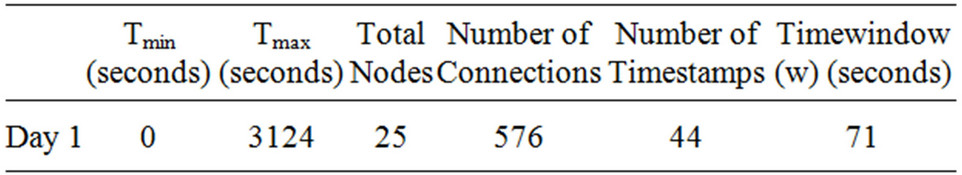
Table 9. RWP_63 Timewindow calculation.

Table 10. INFOCOM’06 static and temporal distance.

Table 11. RWP_98 static and temporal distance.

Table 12. RollerNet static and temporal distance.

Table 13. RWP_63 static and temporal distance.
Since our temporal metric presented gives us a better understanding of the network with respect to the temporal dimension since they can provide us an accurate measure of the delay of the information diffusion process that is not possible with traditional static metrics. The values cannot be directly compared but are good indicators for information diffusion.
4. Adaptive Routing
In this section we present density aware adaptive routing algorithm that integrates forwarding and replication techniques. Here, the threshold is computed based on the average temporal distance gain. It determines sparseness and denseness for given time interval. If the network is dense routing engine uses an encounter based forwarding technique [9], else, it invokes multi period based Spray and Wait [10]. Thus, AR toggles between forwarding and replication technique based on network condition per time window.
4.1. Algorithm
Input:  ,
,  , Average temporal distance Output: Delivery ratio, Overhead ratio Definition: Overhead Ratio = (Relayed Message − Delivered Message)/Delivered Message 1) Read the values of Tmin, Tmax and average temporal distance for INFOCOM’06, RollerNet and RWP.
2) Compute the threshold for the Average temporal distance. At the end of each time stamp calculate the gain of average temporal distance compared to previous timestamp. Threshold = average of all the gain calculated at the end of each timestamp.
3) If average temporal distance < threshold, then do call encounter based forwarding otherwise do call multi period based Spray and Wait.
4) Generate message state report for message traffic vs. Delivery ratio, message traffic vs. Overhead ratio and message traffic vs. Message dropped.
5) Generate comparison chart based on evaluating results.
4.1.1. Encounter base Forwarding
Suppose, node “n” encounters the node “m”, if “n” has a message for “m” then it sends the message to “m”. After that if “n” has a message for the destination id which is stored in summary vector F [] of “m” then “n” forward the message to “m”. Otherwise, if the encounter rate EV of “m” is greater than the encounter rate of “n” then it forwards the message to “m”.
F [ ] = vector of frequently encountered nodes V [ ] = message vector which carries a destination id of the message Wi = current window update interval Upon reception of a Hello message h from node m do ifnewNeighbour(m) == true ifmsgQueue.hasMsgsForDest(m) == true deliverMsgs(m)
updateEV()
for all destinations d ∈n.V[]do if d∈m.f[]
forward message to node m else m.EV>n.EV forward message to node m updateEV()
if time ≥ nextUpdate then EV ← α ・CWC + (1 − α) ・EV CWC ← 0 nextUpdate ← time +Wi end if In this, every node maintains encounter value (EV) and summary vector F[],which stores the frequently encountered node ids. To track a node’s rate of encounter, every node maintains two pieces of local information: EV and current window counter (CWC). EV represents the node’s past rate of encounters as an exponentially weighted moving average, while CWC is used to obtain information about the number of encounters in the current time interval. EV is periodically updated to account for the most recent CWC in which rate of encounter information was obtained. Updates to EV are computed as follows:
EV ← α·CWC + (1 − α)·EV This exponentially weighted moving average places an emphasis proportional to α on the most recent complete CWC. Updating CWC is straightforward: for every encounter, the CWC is incremented. When the current window update interval has expired, the encounter value is updated and the CWC is reset to zero.
4.1.2. Two Period Spray and Wait
It is based on multi period Spray and Wait [11].The algorithm starts with spraying fewer message copies than the copies decided as above, and then waits for a certain period of time to see if the message is delivered. When the delivery does not happen, the algorithm sprays additional copies of a message next period, and again waits for the delivery.
Sprays L1 copies to the network at the beginning of execution and additional L2-L1 copies at next time interval.
TwoPeriodsw(L, α, td )
optcost = L;
for each 0 < L1 < L do L2floor = max[ L+1, L1+(α L1 td (LL1))];
for L2 = L2floor , L2floor +1 do if c2(L1, L2) < opt_cost then opt_cost = c2(L1, L2); opt_cts = [L1, L2]
end if end for end for return opt_cts wheretd = Time deadline L = Number of message copies
α = 0.0015*number of copies L1 = Number of message copies to spray in the first time period L2 = Number of message copies to spray in the second time period c2 = Cost as number of copies used per message
4.2. Simulation setup and Performance Analysis
In our experiments, ONE (Opportunistic Network Environment) [12] simulator is used to evaluate the protocols. This scenario consists of a 4500 × 3400 m area of Helsinki city. These nodes are divided into 6 groups. Group 1 and Group 3 are pedestrian group. Group 2 is automobile group and Group 4, Group 5 and Group 6 are trolleybus group. Pedestrians move with speeds of 0.5 - 1.5 m/s and with waiting time of 0 - 120 seconds. Automobiles move with speeds of 10 - 15 km/h and with waiting time of 0 - 120 seconds. Trolleybuses move with speeds of 7 - 10 km/h and with waiting time of 10 - 30 seconds at every station. Two kinds of devices are used in the experiments. One is Bluetooth device which transmission range is 10 m and transmission speed is 2 Mbps. The other is 802.11b WLAN device which transmission range is 30 m and transmission speed is 4.5 Mbps. The buffer of these mobile devices is up to 1 MB. When buffer is full, new messages will not be accepted by the node until some old messages are deleted from the buffer. The duration of the simulation is 43,000 simulation seconds.
Assumptions
It is assumed that the network is congestion free and node have infinite energy. Default buffer management policies are used. No explicit settings made to schedule and drop policies.
Datasets
Real and Synthetic datasets are used for simulation. For, the real trace file INFOCOM’06 and RollerNet trace files are used. For synthetic data RWP model is used. Information about the name, location, duration, participants and address IDs are summarized in Tables 2-5. First temporal distance of real traces and synthetic datasets are evaluated and presented in Tables 10-13. Real trace are first converted to ONE compatible format and then imported for simulation. RWP dataset is generated using ONE simulator.
Performance Metrics
Delivery Probability: The delivery probability is a measure of the fraction of the created packets that are delivered to the destination. This is the ratio of the total number of packets that are delivered to their destination to the total number of packets that are created.
Overhead Ratio: The overhead ratio is calculated using the following equation.
Here, the term relayed messages refers to the messages that have been forwarded from the source to an intermediate node to be forwarded towards the destination. This number is a measure for the number of packets or copies of packets that have been inducted into the network. The number of delivering messages refers to the total number of creating packets that are successfully delivered to the destination.
INFOCOM’06
Delivery ratio, overhead ratio and number of dropped messages comparison for AR, Epidemic and PRoPHeT routing with INFOCOM’06.
As shown in Figure 2 the delivery ratio of AR observed better compared to Epidemic and ProPHeT. But, overall value is still poor. This is due to INFOCOM 2006 had a smaller number of timestamps and larger time window size compared to RWP. Hence, AR with INFOCOM’06 executed forwarding and replication all most same number of times.
Figure 3 indicates that AR has a low overhead ratio due almost the same number of time forwarding and replication executed. Thus, in forwarding numbers of transmissions are less and resulting in a limited message compared to the Epidemic and ProPHeT. Where in Epidemic is purely replication and ProPHeT is probability based multi copy scheme.
Number of message dropped in AR is low compared to ProPHeT and Epidemic. Since, in forwarding phase node’s encounter rate checked and in replication two

period Spray and Wait used. This resulted in dropping the less number of messages as shown in Figure 4.
RollerNet
As shown in Figure 5 RollerNet traces have the number of connections. Thus created more contact opportunities. AR calls more number of times forwarding which result lesser message drop and better delivery ratio.
In a RollerNet numbers of connections are high compared to RWP. Thus, the network is dense and AR frequently executed forwarding technique. This resulted in lower overhead as presented in Figure 6.
AR in forwarding phase uses encounter based technique. Thus due to higher contacts opportunities forwarding is frequently called. Hence, the numbers of dropped

Figure 2. Delivery Ratio Comparison of AR, Epidemic and ProPHeT.

Figure 3. Overhead Ratio Comparison of AR, Epidemic and ProPHeT.

Figure 4. Number of Dropped Messages Comparison of AR, Epidemic and ProPHeT.
messages are zero and results in minimum overhead as shown in Figure 7.
5. Conclusion and Future Work
It reveals that the node mobility plays a vital role in the efficient diffusion of information in challenging environment. And while doing so one cannot ignore to understand the movement patterns and related properties such as time order, frequency, contact duration, inter-contact time, etc. These properties are applied in designing an efficient routing in IC-MANET. And understanding the dynamics of the network and thereby taking forwarding

Figure 5. Delivery Ratio Comparison of AR, Epidemic and ProPHeT.

Figure 6. Overhead Ratio Comparison of AR, Epidemic and ProPHeT.

Figure 7. Number of Dropped Messages Comparison of AR, Epidemic and ProPHeT.
or replication decisions. It is established that routing efficiency terms of delivery ratio and overhead are significantly improved with temporal metrics. In future, it can be extended for contact sequence based probabilistic routing and temporal closeness centrality based evaluations.
6. Acknowledgements
We express our sincere gratitude to the management of Ganpat University—Mehsana and Marwadi Education Foundation—Rajkot; for providing us research opportunities and their wholehearted support for such activities.
REFERENCES
- T. Spyropoulos, K. Psounis and C. S. Raghavendra, “Single-Copy Routing in Intermittently Connected Mobile Networks,” The First Annual IEEE Communications Society Conference on Sensor and Ad Hoc Communications and Networks, 4-7 October 2004, pp. 235-244.
- K. Fall, “A Delay-Tolerant Network Architecture for Challenged Internets,” Proceedings of the 2003 Conference on Applications, Technologies, Architectures, and Protocols for Computer Communications, 2003, pp. 27- 34.
- V. Kostakos, “Temporal Graphs,” Physica A: Statistical Mechanics and Its Applications, Vol. 388, No. 6, 2009, pp. 1007-1023.
- J. Tang, M. Musolesi, C. Mascolo and V. Latora, “Characterising Temporal Distance and Reachability in Mobile and Online Social Networks,” ACM SIGCOMM Computer Communication Review, Vol. 40, No. 1, 2010, pp. 118-124. doi:10.1145/1672308.1672329
- E. Nordström, P. Gunningberg and C. Rohner, “Haggle: A Data-Centric Network Architecture for Mobile Devices,” Proceedings of the 2009 MobiHoc S3 Workshop on MobiHoc S3, 2009, pp. 37-40.
- P.-U. Tournoux, J. Leguay, F. Benbadis, J. Whitbeck, V. Conan and M. Dias de Amorim, “Density-Aware Routing in Highly Dynamic DTNs: The RollerNet Case,” IEEE Transactions on Mobile Computing, Vol. 10, No. 12, 2011, pp. 1755-1768. doi:10.1109/TMC.2010.247
- F. Bai and A. Helmy, “IMPORTANT: A Framework to Systematically Analyze the Impact of Mobility on Performance of Routing Protocols for Adhoc Networks,” 22nd Annual Joint Conference of the IEEE Computer and Communications Societies, Vol. 2, 30 March 2003-3 April 2003, pp. 825-835.
- J. Tang, M. Musolesi, C. Mascolo and V. Latora, “Temporal Distance Metrics for Social Network Analysis,” Proceedings of the 2nd ACM workshop on Online Social Networks, 2009, pp. 31-36.
- J. Zhang, G. Luo, K. Qin and H. Sun, “Encounter-Based Routing in Delay Tolerant Networks,” International Conference on Computational Problem-Solving (ICCP), Chengdu, 21-23 October 2011, pp. 338-341. doi:10.1109/ICCPS.2011.6089802
- E. Bulut, Z. Wang and B. K. Szymanski, “Cost Efficient Erasure Coding Based Routing in Delay Tolerant Networks,” IEEE International Conference on Communications, 2010, pp. 1-5. doi:10.1109/ICC.2010.5502382
- E. Bulut, Z. Wang, and B. K. Szymanski, “Cost-Effective Multiperiod Spraying for Routing in Delay-Tolerant Networks,” IEEE/ACM Transactions on Networking, Vol. 18, No. 5, 2010, pp. 1530-1543. doi:10.1109/TNET.2010.2043744
- A. Keränen, T. Kärkkäinen and J. Ott, “Simulating Mobility and DTNs with the ONE (Invited Paper),” Journal of Communications, Vol. 5, No. 2, 2010, pp. 92-105.