Journal of Mathematical Finance
Vol.2 No.2(2012), Article ID:19211,18 pages DOI:10.4236/jmf.2012.22016
Interest Rate Models
1Department of Accounting and Finance, University of Manitoba, Winnipeg, Canada
2Department of Statistics, University of Manitoba, Winnipeg, Canada
Email: thava@temple.edu
Received December 15, 2011; revised January 14, 2012; accepted January 25, 2012
Keywords: affine process; dynamic term structure models; jump-diffusions; quadratic-Gaussian DTSMs
ABSTRACT
In this paper, we review recent developments in modeling term structures of market yields on default-free bonds. Our discussion is restricted to continuous-time dynamic term structure models (DTSMs). We derive joint conditional moment generating functions (CMGFs) of state variables for DTSMs in which state variables follow multivariate affine diffusions and jump-diffusion processes with random intensity. As an illustration of the pricing methods, we provide special cases of the general formulations as examples. The examples span a wide cross-section of models from early one-factor models of Vasicek to more recent interest rate models with stochastic volatility, random intensity jump-diffusions and quadratic-Gaussian DTSMs. We also derive the European call option price on a zero-coupon bond for linear quadratic term structure models.
1. Introduction
In this review, we summarize available continuous time technology for pricing default-free term structures. Our main goal is to provide a unified approach to the pricing exercise based on well-developed application of stochastic calculus to finance problems. In our discussions, we always start from state variable processes given under a risk-neutral measure. We make no attempt to systematically present the transition between the actual measure and the risk-neutral measure. Thus, we leave out the question of reconciling time series properties of the underlying state variables (such as short rate), which are defined under the actual measure, and the properties of the market yields (or, equivalently, bond prices), which are derived under the risk-neutral measure.
We begin with affine diffusion models of interest rates. The menu of available models in this class is truly vast.1 The most redeeming features of this class of models are the availability of closed form solutions for derivatives on the short rate and the ability of models to reproduce a variety of term structure patterns. Models in this class have closed form solutions for bond and bond option prices, which makes them particularly attractive for empirical work. Some models in this class, especially twoor three-factor models, are flexible enough to have a satisfactory fit to observed term structures. The last property is essential for pricing options on bonds. Extended versions of Vasicek and CIR (e.g., [2,5,14]) allow for timevarying coefficients in state variable dynamics. This extra feature allows the model to fit the initial term structure.
Discontinuous movements in interest rates are caused by central banks and unexpected news announcements. In order to implement a specific policy, monetary authorities often use specific rate-setting rules which result in entire yield curve shifts in line with movements in the benchmark rate. Empirical evidence suggests that interest rates exhibit substantial skewness and kurtosis, and hence jump-diffusion interest rate models are more appropriate2. In deriving the term structure of spot rates for the case of discontinuous interest rates, we stay within the affine jump-diffusion class of models. The bond prices are still available in near-closed form up to the solutions of Riccati ordinary differential equations for the coefficients of the conditional moment generating function of the state variables.
Market spot rates are mostly positive, and a class of quadratic interest rate models is designed to restrict spot rates to be positive without ruining the bond price tractability. Square-Gaussian models, in which the short rate is a sum of squares of Gaussian state variables, have been investigated by [28-30]. The models of Quadratic-Gaussian class were studied by [31-35]. The mathematics of these models is similar to that of affine jump diffusions and also allows closed form solutions for bond prices in the exponential quadratic form.
Previous jump-diffusion TSMs treat short rate intensity in one of the following restrictive ways:
1) A deterministic function of the short rate ([26]);
2) Constant except for FOMC meeting days and macroeconomic news announcements, in which case it is a linear function of short rate, interest rate volatility, and Fed rate target; or 3) A function of the spread between the Fed funds rate and the target.
Thus, we also consider a recent extension of a class of Linear-Quadratic term structure models (LQTSMs) to a class of jump-diffusion TSMs in which short rate jump intensity follows its own stochastic process (see [36-38] for details). We show how this model class is designed to have a closed form conditional moment generating function and bond prices. Despite strong restrictions on state variable processes that are necessary to obtain closed form bond prices, [36] shows that the inclusion of random intensity improves the model fit to both the dynamics of the term structure and that of the volatility term structure. The main mechanism of improved fit is the short term kurtosis of the short rate.
The rest of this paper is organized as follows. In Section 2, we present a general technique of solving for joint CMGF of an affine state vector and its integral. Special cases include CMGF of an affine vector and bond prices within affine model class. Section 3 covers affine jumpdiffusion DTSMs. Finally, we close with a review of quadratic Gaussian models and a more general class of linear quadratic class of DTSMs with jumps of random intensity. We also derive the price of a European call option using a generalized transform.
2. Affine Term Structure Models
In this section we provide general results for affine models. As an illustration, we also give detailed account of some popular special cases.
Definition. Let  be a vector of
  state variables, and let
  be the short rate. A model is affine if the state vector solves the following diffusion SDE:
 (2.1)
(2.1)
 (2.2)
(2.2)
where ,
,  ,
,  (constant matrix),
  ,
,  ,
,  is a diagonal
  -matrix such that
 , and
, and  is a vector of standard Wiener processes. We assume that an equivalent martingale measure (EMM) exists, and all processes and expectations (unless stated otherwise) are understood as those under the EMM, e.g., the process in (2.1) is written under the EMM. The SDE (2.1) implies that the joint conditional moment generating function (CMGF) of the state vector is exponential affine:
 (2.3)
(2.3)
where .
.
The following lemma is a special case of [39] with no jumps.
Lemma 2.1. Assume that a state vector Y satisfies (2.1). Consider the following boundary value problem:
 (2.4)
(2.4)
 (2.5)
(2.5)
This problem has a stochastic solution of the form3
 (2.6)
(2.6)
with the following initial conditions:  and
and  .
.
Proof. Applying Ito’s lemma to function
 , we have4

After taking the conditional expectation of both sides and noting that the first of the two integrals on the right hand side is zero due to (4), we have

In order to prove the exponential affine form of the solution (2.6) to (2.4), it suffices to use it as a guess and find the equations determining  coefficients
  and
and . Substitution of
  into (2.4) produces the following equation that must hold for any value of the state vector:

The left hand side of the above equation is an affine function in . Since the equation must hold for arbitrary vector
 , both coefficients of the affine function must be zero. This requirement gives two Riccati ODEs for coefficients
  and
and :
:
 (2.7)
(2.7)
 (2.8)
(2.8)
where  and
and  can be inferred from the following expression:

It follows from (2.5) that the initial values are  and
and .
.
The expression for MGF for an affine diffusion is just a special case of the above result for :5
:5
 (2.9)
(2.9)
The coefficients satisfy the following Riccati ODEs:


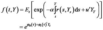
Zero coupon bond prices are a special case of the Lemma. Assuming again that the short rate process is affine in the state variables as given in (2.2), the price of a zero-coupon default-free bond with maturity  and face value of $1 is given by
 (2.10)
where the expectation is under a EMM. The expectation in (2.10) is a special case of (2.6) with  and
and . Given these restrictions, the bond price has exponential affine form

and satisfies the following PDE:
 (2.11)
Bond price coefficients  and
and  solve the following system of Riccati equations (a special case of (2.7)-(2.8)):
 (2.12)
 (2.13)
 (2.14)
The spot rate is given by
 (2.15)
Taking limits as , we obtain the short rate
  (which is also given in (2.2))

2.1. One-Factor Interest-Rate Models
In this section we provide closed form expressions of the default-free bond prices with details. Under the EMM, the evolution of this process is described by a diffusion Gauss-Markov process of the form:
 (2.16)
where  is a standard Brownian motion and
 ,
,  are suitable processes adapted to
  . The usual assumption is that
  and
and  are simply functions of the short rate
  and time
 , i.e.,
  and
and  .
.
Theorem 2.2. Consider the Hull and White model of the form
 (2.17)
where ,
,  and
and  are non-random functions of
  such that
 (2.18)
The price at time  of a zero-coupon default free bond paying $1 at time T is
 (2.19)
where


Note: The Merton [43] model, Vasicek [1] model, and the Ho-Lee model [44] are special cases of (2.17).
Proof. Under these assumptions (2.18) the equation (2.17) has a unique (strong) solution

Since  is the Markov process, it follows that

where  is conditionally normal. The conditional mean, variance, and the Laplace transform are given as:


and

Hence the default-free time  bond price is given by

Note 1. The Vasicek model is a special case with constant coefficients:  and
and  (
( ), such that
 . It follows from Theorem 2 that
 (2.20)
 (2.21)
Note 2. For the extended Vasicek model,  ,
,  , it follows from Theorem 2.2 that
 (2.22)
 (2.23)
Theorem 2.3. Consider the Cox, Ingersoll and Ross (CIR) model, the interest rate process  is given by

where  is given. The price at time
  of a zerocoupon bond paying $1 at time t is

where


and .
.
Proof. See the Appendix.
2.2. Multi-Factor TSMs
There is substantial evidence that bond yields have timevarying conditional volatilities (see, e.g., [45,46]). Even though general single-factor DTSMs do have built-in time varying bond yield volatilities (except for basic Gaussian affine and lognormal models), however, they can not match the variation observed in practice. For example, single-factor models tend to understate the volatility of long-term yields, overstate the correlation between yields of different maturities, require mean reversion properties that cannot simultaneously match cross section and time series of bond yields. There is also evidence that linear drift term in single factor models is misspecified. Multifactor models are designed to address some of these issues.
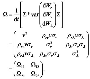
Here, we give an example of a three-factor affine family model presented in [11]. The short rate is a CIR process with long run mean (central tendency) following Ornstein-Uhlenbeck process and stochastic volatility following a CIR process all under an EMM. The state vector  is defined as follows:


where , and all other correlations are zero.
According to (2.11), the price of a zero coupon bond in this model satisfies the following PDE:

Since the model is in the affine category, we look for a solution in the following form:

where vector  has three components
 and
and . The Riccati equations (2.12) and (2.13) along with the boundary conditions (2.14) imply
 (2.24)
 (2.25)
 (2.26)
 (2.27)
 (2.28)
Solutions to equations (2.25) and (2.26) are available in closed form:


Explicit solutions for  and
and  are not available. However, numerical solutions are easy to obtain.
3. Affine Jump-Diffusion DTSMs
There is a growing body of empirical research showing that discontinuous behavior of interest rates is essential in correctly describing their distribution and fitting terms structures to the data. e.g., [24-26] all find that introducing jumps substantially improves the fit of the conditional distribution of short-term interest rates compared to that of nested diffusion models.6
The relative scarcity of empirical work on models of discontinuous interest rates is most likely related to far less tactable mathematics involved in these models. Interest rates are mean reverting. In general, the mean reversion feature combined with jumps in the interest rates makes the moments of jump-diffusion distribution dependant on the timing of the jumps. However, in jumpdiffusion models it turns out that the density of equity returns does not depend on the jump times. In order to derive the expression for the CMGF of the state variables and bond prices for the case of affine jump diffusion we generalize the Lemma 2.1 in order to include jumps. The CMGF for a jump-diffusion process turns out to be the product of CMGFs of continuous and jump parts of the processes.
Definition. Let Y be a vector of n state variables and r is the short rate. A model is affine if the state vector solves the following diffusion SDE:
 (3.1)
(3.1)
where ,
,  ,
,  constant matrix,
  ,
,  ,
,  is a diagonal
  -matrix such that
 ,
,  is a vector of standard Wiener processes,
  is a Poisson counter with state-dependent intensity, a positive affine function of
 ,
,  , and
, and  is a jump size with time-homogeneous MGF
 . We assume that jump size and jump arrival times are uncorrelated with the diffusion part of the process. In general, jump sizes can be correlated across different state variables.
As before, (2.2) is the expression for the short rate. We again assume that an equivalent martingale measure (EMM) exists, and all processes and expectations (unless stated otherwise) are understood as those under the EMM. The SDE (3.1) implies that the joint conditional moment generating function (CMGF) of the state vector is exponential affine. To see why this is the case, we extend the lemma of section 2 to include jumps.
Lemma 3.1. Assume that a state vector Y satisfies (3.1). Then, the joint CMGF of process  and its integral is given by the following expression
 (3.2)
(3.2)
where . This CMGF solves the following boundary value problem:
 (3.3)
(3.3)
 (3.4)
(3.4)
where
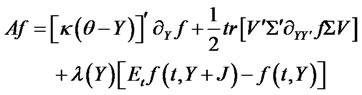 (3.5)
(3.5)
is the infinitesimal generator of state variable vector  applied to the function f. Coefficients
  and
and  satisfy the following ODEs:
 (3.6)
(3.6)
 (3.7)
(3.7)
 (3.8)
(3.8)
Proof. The proof is somewhat similar to the proof of Lemma 2.1 To find equations for the coefficients  and
and , we insert exponential affine solution expression (3.2) into (3.3). The resulting expression

must hold for all values of the state variables, which results in ODEs (3.6)-(3.8).
3.1. One-Factor Jump-Diffusion Vasicek Model
The valuation of fixed income securities requires transition from actual to EMM measure. In general, this task can be accomplished by specifying a stochastic discount factor (SDF) for the economy. In continuous time, the SDF,  , places a restriction on a price
  of a zerocoupon bond according to the following Euler condition (see [47]):
In a model adapted from [22], the SDF satisfies a jump-diffusion SDE:
 (3.9)
(3.9)
where  is the price of diffusion risk,
  is the price of jump risk,
  is a demeaned (compensated) Poisson process with intensity
  jumps per year. They also assume that the sort rate follows O-U process with jumps:

The zero-coupon bond price, being a function of time,  , and the short rate,
  , satisfies the following Ito SDE:

Define  and substitute the above differential into the Euler condition to obtain the following PDE for the zero-coupon bond price:

(3.10)
 (3.11)
The resulting PDE describes the evolution of the bond price under EMM. Under this risk-neutral measure the short rate process satisfies


The transformed counting process has new risk-adjusted intensity . The PDE (3.11) belongs to a class that generates exponential-affine bond prices. Thus, we look for a solution to the bond price in the following form:

Inserting this expression into the PDE, we have

where  is the MGF of the jump size. The above expression is an identity that must hold for any values of time and short rate. This requirement leads to separate ODEs for coefficients A and B:
 (3.12)
 (3.13)
 (3.14)
The terminal condition (3.14) follows from the fact that the bond has face value of $1 at maturity. Subject to (3.14), solutions to (3.12)-(3.13) are given by


3.2. One-Factor Cox-Ingesoll-Ross Model with Jumps
[4] develops a general equilibrium model for a standard economy with a representative agent with log-utility preferences, and shows that the short rate is a linear function of the single state variable that drives the economy. The short rate therefore inherits the same dynamic properties as the state variable and follows the square root SDE7 (in this case, we also augment it with a jump-diffusion component; see also [15]):
 (3.15)
According to the first fundamental theorem of finance, discounted prices are martingales. Thus, a zero-coupon bond price satisfies the following PDE:

where  is the infinitesimal generator of the short rate (3.15):

The relation between risk neutral and actual measure parameters is based on the CIR pricing kernel:


where ,
,  and
and
 . Substituting a solution of the form
 into the above PDE, just like in the one-factor Vasicek model, we obtain two separate ODEs for the functions
  and
and :
:


Integrating the two ODEs, we have the solution for the CIR zero-coupon bond price with jumps in the short rate:

where
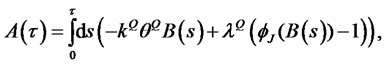
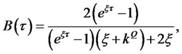
and

3.3. A Two-Factor Vasicek Model with Jumps in the Long-Run Mean
In this two-factor model, the two state variables are the short rate,  , and the central tendency (long-run mean) of the short rate,
 . We assume as before that both risks are priced as follows:

where parameters have the same definitions as in (3.19). Under the EMM, the short rate follows a standard Vasicek model, and the long run-mean of the short rate is given by a pure jump process:

and

The corresponding PDE for a zero-coupon bond price:
 (3.16)


Since we are dealing with an exponential affine model once again, we can write the solution as

Substituting this solution into (3.16), the PDE breaks down into three separate ODEs for functions ,
,  , and
, and :
:

The functions  and
and  are given by:
 and
and . Moreover, the function
  can be obtained numerically by using
 (3.17)
Note: When the jump size is normally distributed with mean , variance
 , and MGF

by using the following first-order Taylor series approximation as in [18]8,

the function (3.17) turns out to be:

Under the normality assumption of the jump sizes, the closed-form approximate solution for bond prices becomes very useful for calibration, estimation and testing.
4. The Quadratic Model
The common problem with most interest rate models is that interest rates can become negative (except in CIRtype models). Even though negative interest rates are not impossible, they are rare. This fact has led to the need to develop models of interest rates that guarantee positive rates. The models in this category are numerous.9 However, most of these early models suffer from various problems. e.g., a rational log-normal model of [48] suffers from calibration problems in that bond prices and short rates are bounded both from below and above. As a result this model is arbitrage free only for a finite period of time. This restriction proves too binding in empirical work. Other ways of guaranteeing positive rates is to transform the state variable. Popular class of models that achieve that is log-r models. The short rate is the exponent of a state variable ,
,  , which follows an extended Vasicek process. Historically, due to availability of easy lattice implementation tools, the two most widely used models in this class are [51,52]. However, this transformation presents theoretical problems. The problem with these models is that the expected future value of the risk-free bank account
 even for arbitrarily small
(see [53]).
4.1. Quadratic-Gaussian Interest Rate Models
Recently, more attention has been paid to a different specification, quadratic-Gaussian, that guarantees positive rates, does not suffer from these problems, and still tractable enough to generate near closed form bond and in some cases even bond option prices. The simplest form of this model is the so-called square Gaussian model in which the short rate is simply the sum of squares of the state variable.10 A more general model is in the Quadratic-Gaussian (QG) class with the short rate a general quadratic form of the state variables, which follow a process with affine drift and constant volatility. In an n-factor Quadratic-Gaussian model the short rate is
 (4.1)
(4.1)
where ,
,  , and
, and . The state variables
  follow an n-dimensional Gaussian process under a risk neutral measure:
 (4.2)
(4.2)
where ,
,  ,
,  constant matrix, and
  is a vector of standard Wiener processes. We can always rewrite the short rate in (4.1) in the following form after shifting the state variable
  by a constant vector:

The state SDE (4.2) does not change from this transformation except for obvious redefinition of parameters. Quadratic-Gaussian models have been studied by [28, 31-35,38,54,55]11 Similarly to affine models, we look for the zero coupon bond price solution to (2.10) in the following form:
 (4.3)
(4.3)
where  is
is  matrix. The bond price satisfies PDE (2.4) with
  and
and . Using (4.3) in (2.4), we obtain the following PDE:

Since this equation has to hold for any values of the state variables, it separates into three independent Riccati ODEs for ,
,  , and
, and :
:


Moreover, if the matrix  is symmetric, the system reduces to


Example 1. For a one-factor square-Gaussian model of interest rates considered in [6] and [5]:

 (4.4)
(4.4)
For this model, the bond prices, as well as bond option prices, have closed form expressions given by the following:
1) The zero coupon bond price is

where


and

2) The European call option price with maturity  and strike
  written on a zero-coupon bond with maturity
  is given by

with parameters given by the following expressions:


4.2. Linear-Quadratic Interest Rate Model
The difficulty of fitting term structures of interest rates with diffusion models has led to the study of the impact of jumps in the interest rates on spot rate properties. [25, 26,37,57,58] point out that including jumps in a model helps better explain properties of various interest rates. When extending a model in any way, we are also concerned about whether the model will still have a closed form solution for bond prices, bond option (cap, floor, swaption) prices, and whether the extension helps improve the fit of volatility term structures to those implied by swaptions and caps when the simpler model has failed to do so. In the case of including jumps into diffusion models, [59] use three years of interest rate cap price data and show that within a three factor SVJ DTSM significant negative jumps in interest rates are required to fit implied volatility smile.
[36] argue that most of the previous research is too restrictive in the way it treats jump intensity. Usual assumptions range from constant intensity to a rather restrictive functional form of underlying state variables that may include economic variables as in [37]. [36] introduce a new class of interest rate models, linear-quadratic term structure model (LQTSM). The new feature is that jump intensity is now a separate state variable that follows it own SDE. In their empirical implementation, they use essentially a 3-factor model with the state vector that includes the short rate, the random volatility, and the stochastic intensity. The rate on 3-month T-bills serves as a proxy for the short rate. To estimate parameter values [36] relies on generalized method of moments (GMM) approach of [60]. At each iteration of the GMM optimization routine, however, they have to compute the remaining two latent state variables, volatility and intensity, for every date of their dataset. They do it by resorting to the so-called implied-state GMM (IS-GMM) procedure of [61]. For given parameter values at each iteration they use high frequency futures market data on the changes in T-Bill yields to compute conditional variance and kurtosis. Stochastic volatility and intensity are then identified from these two higher moments. They find that introducing random intensity substantially improves both the model fit (through better fit of short term kurtosis) as well as the dynamics of the interest rate volatility term structure. In a VAR model run on daily data they also establish that jumps are not only associated with macroeconomic announcements or FOMC meeting dates but also with unanticipated news.
Below, we show how LQTSM class is designed to have a closed-form solution, and we give a simple example of a special case closely related to the SVJT model that [36] studies. We start with the extended transform (2.6). LQTSM class is designed (or defined) to have the following exponential LQ form for extended transform12:
 (4.5)
(4.5)
 (4.6)
(4.6)
 (4.7)
(4.7)
where  is a vector of state variables,
  ,
,  is jump intensity, jump size vector
  with time-homogeneous MGF
 , the mean of the jump size vector
 ,
,  ,
,  is a vector of standard Wiener processes, Poisson process
  is independent of jump size and of the diffusion vector W,
  ,
,  , and
, and  [36] derives risk-neutral corrections to model parameters based on power-utility pricing kernel by following the approach of [4,38]. We skip this stage in the derivation and assume that all processes are already expressed under an EMM. Extended transform (4.5) must satisfy the following PDE:
 (4.8)
(4.8)
 (4.9)
(4.9)
 (4.10)
where  is the value of the state vector immediately after a jump. Similar to affine JD models, the expectation in the integro-differential equation (4.8) should break up into the product of the MGFs for continuous and discontinuous parts of the state vector process as these parts are assumed independent in this specification. The only complication is the quadratic form in the definition of extended transform for LQTSM class in (4.5). [36] works around this complication by assuming that in the state vector only a subvector of, say, the first
  components is discontinuous, i.e., follows a JD process. The remaining
  components are diffusions:


The extended transform (4.5) must be exponential quadratic only in :
:
 (4.11)
In order to obtain separate ODEs for three functions , and
, and , the next obvious requirement is that once we substitute (4.11) into (4.8) there must be no terms other than affine in
  (i.e.,
 ) and quadratic in
  (i.e.,
 ). Then, the functional forms of the short rate,
  , intensity,
  , and drift and diffusion coefficients of the transition equation (4.6) are dictated by the above requirement. For example, the second term in PDE (4.8) contains the gradient of the transform and the jump part is proportional to
 :
:

These functional forms of the gradient and the jump term jointly imply that the first  components of vector
  in (4.6) and intensity
  must be
  and
and  and the last
  components of vector
  must be
 :
:


Just like , the short rate (last term in the PDE) must be
  and
and :
:

with obvious definitions for . Further, the trace part of the PDE has the following form:

where  is a symmetric matrix. The above expression implies that

and

Substituting (4.11) into PDE (4.8) we have the following identity that must hold for all :
:

where

Terms independent of , affine in
 , affine in
 , and quadratic in
  must each be equal to zero in this identity. This restriction results in a system of four ODEs for functions
 ,
,  ,
,  , and
, and . For details, the reader can consult [36]. The initial conditions are


The zero coupon bond price has the same form as in (4.5) with .
.
Example (LQTSM of [36]). Assume that the state vector consists of short rate, volatility, and random jump intensity. These three state variables are assumed to solve the following transition equations:
 (4.12)
with the following definitions and notation:


We look for a zero coupon bond price in the following form:
 (4.13)
As in [36] we assume that  is symmetric. In the Appendix we derive the following ODEs for functions
 ,
,  ,
,  , and
, and 
 (4.14)
 (4.15)
 (4.16)
 (4.17)
subject to the following initial conditions:
 (4.18)
 (4.19)
Here,  is the moment generating function of the jump size.
In order to conclude the discussion of LQTSMs, we derive the price of a European call option from a generalized transform using a technique similar to the one used by [39,62,63]. We are looking for the price of a European call option on a zero coupon bond. The call has  years to maturity and a strike price,
 . The zero-coupon bond has maturity date,
  , the face value of
 , and the current price
 . We provide the derivation of the option price for the 3-factor LQTSM from [36] given in the above example. We assume that the state dynamics in (4.12) are given under an EMM. The value of the European call option is given by the following risk neutral expectation with respect to (4.12):
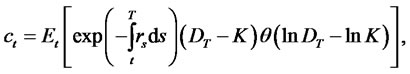 (4.20)
where  is the Heaviside function defined as

In order to handle the truncation under the expectation in (4.20), we use a well known complex integral representation of the Heaviside function

Using this representation we write the call price as (4.21)
where
 (4.22)
and ,
,  To complete the derivation, we use a well-known result from the theory of generalized functions:
 (4.23)
where  is the principal value of the integral over
 :
:

Each term in (4.23) is understood as a linear functional acting on a finite infinitely differentiable function :
:

where we use the fact that the principal value of the integral over  vanishes as this function is odd. Subtracting
  from the integrand makes it regular, does not require principal value specification, and is suitable for numerical integration.
The expression for the call price can now be written as follows:

where

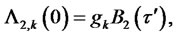
Function  in (4.22) can be viewed as a generalized transform for the zero coupon bond yield. Since we already have the result for the bond price for the LQTSM class, we look for the expectation in (4.22) in the exponential quadratic form: (4.24)
Here,  is the time remaining to the bond’s maturity at the time the option matures. Recall that
  is the time remaining to the maturity of the option as of today’s date
 . For a given
 , the four functions in (4.24),
  (
( ), satisfy the same Riccati ODEs (11)-(16) as
 ,
,  ,
,  , and
, and , respectively, and the following initial conditions:


|
|
 (4.21)
 (4.24)
where 
Since numerical analysis of option prices and Greeks for hedging purposes is beyond the scope of this paper, we refer the reader to the following work on this topic. In [64,65], authors compute European option prices and the Greeks. For a model of an underlying asset process they use a theoretically attractive Variance-Gamma process. They estimate gradients of a European call option by Monte Carlo simulation methods. In computing the gradients, they compare the efficiency of indirect methods (finite difference techniques) and direct methods (infinitesimal perturbation analysis and likelihood ratio).
REFERENCES
- O. Vasicek, “An Equilibrium Characterization of the Term Structure,” Journal of Financial Economics, Vol. 5, No. 2, 1977, pp. 177-188. doi:10.1016/0304-405X(77)90016-2
- J. C. Hull and A. D. White, “Pricing Interest-Rate-Derivative Securities,” Review of Financial Studies, Vol. 3, No. 4, 1990, pp. 573-592. doi:10.1093/rfs/3.4.573
- J. C. Hull and A. D. White, “One-Factor Interest-Rate Models and the Valuation of Interest-Rate Derivative Securities,” Journal of Financial and Quantitative Analysis, Vol. 28, No. 2, 1993, pp. 235-254. doi:10.2307/2331288
- J. C. Cox, J. E. Ingersoll and S. A. Ross, “A Theory of the Term Structure of Interest Rates,” Econometrica, Vol. 53, No. 2, 1985, pp. 385-407. doi:10.2307/1911242
- F. Jamshidian, “A Simple Class of Square Root Interest Rate Models,” Applied Mathematical Finance, Vol. 2, No. 1, 1995, pp. 61-72. doi:10.1080/13504869500000004
- A. Pellser, “Eccient Method for Valuing and Managing Interest Rate and Other Derivative Securities,” Ph.D. Thesis, Erasmus University, Rotterdam, 1996.
- F. A. Longsta, “The Valuation of Options on Yields,” Journal of Financial Economics, Vol. 26, No. 1, 1990, pp. 97-121. doi:10.1016/0304-405X(90)90014-Q
- F. A. Longsta and E. S. Schwartz, “Interest Rate Volatility and the Term Structure: A Two-Factor General Equilibrium Model,” The Journal of Finance, Vol. 47, No. 4, 1992, pp. 1259-1282. doi:10.2307/2328939
- R. R. Chen and L. O. Scott, “Pricing Interest Rate Options in a Two-Factor Cox-Ingersoll-Ross Model of the Term Structure,” Review of Financial Studies, Vol. 5, No. 4, 1992, pp. 613-636. doi:10.1093/rfs/5.4.613
- P. Balduzzi, et al., “Stochastic Mean Models of the TermStructure of Interest Rates,” In: B. Tuckman and N. Jegadeesh, Eds., Advanced Tools for the Fixed-Income Professional, Wiley, Chichester, 2000.
- P. Balduzzi, et al., “A Simple Approach to Three-Factor Affine Term Structure Models,” The Journal of Fixed Income, Vol. 6, No. 3, 1996, pp. 43-53. doi:10.3905/jfi.1996.408181
- L. Chen, “Interest Rate Dynamics, Derivatives Pricing, and Risk Management,” Lecture Notes in Economics and Mathematical Systems, Vol. 435, 1996. doi:10.1007/978-3-642-46825-4
- J. James and N. Webber, “Interest Rate Modelling,” John Wiley & Sons, New York, 2000.
- Y. Maghsoodi, “Solution of the Extended CIR Term Structure and Bond Option Valuation,” Mathematical Finance, Vol. 6, No. 1, 1996, pp. 89-109. doi:10.1111/j.1467-9965.1996.tb00113.x
- C. M. Ahn and H. E. Thompson, “Jump-Diffusion Processes and the Term Structure of Interest Rates,” The Journal of Finance, Vol. 43, No. 1, 1988, pp. 155-174. doi:10.2307/2328329
- S. H. Babbs and N. J. Webber, “Term Structure Modelling Under Alternative Official Regimes,” In: M. Dempster and S. Pliska, Eds., Mathematics of Derivative Securities, Cambridge University Press, Cambridge, 1998, pp. 394-422.
- D. Backus, S. Foresi and L. Wu, “Macroeconomic Foundations of Higher Moments in Bond Yields,” New York University, New York, 1997.
- J. Baz and S. R. Das, “Analytical Approximations of the Term Structure for Jump-Diffusion Processes: A Numerical Analysis,” The Journal of Fixed Income, Vol. 6, No. 1, 1996, pp. 78-86. doi:10.3905/jfi.1996.408164
- G. Chacko, “A Stochastic Mean/Volatility Model of Term Structure Dynamics in a Jump-Diffusion Economy,” Harvard University, Cambridge, 1996.
- S. R. Das, “A Direct Discrete-Time Approach to Poisson-Gaussian Bond Option Pricing in the Heath-JarrowMorton Model,” Journal of Economic Dynamics and Control, Vol. 23, No. 3, 1998, pp. 333-369. doi:10.1016/S0165-1889(98)00031-1
- S. Das, “Discrete-Time Bond and Option Pricing for JumpDiffusion Processes,” Review of Derivatives Research, Vol. 1, No. 3, 1997, pp. 211-243. doi:10.1007/BF01531143
- S. R. Das and S. Foresi, “Exact Solutions for Bond and Option Prices with Systematic Jump Risk,” Review of Derivatives Research, Vol. 1, No. 1, 1996, pp. 7-24. doi:10.1007/BF01536393
- S. Heston, “A Model of Discontinuous Interest Rate Behavior, Yield Curves, and Volatility,” Review of Derivatives Research, Vol. 10, No. 3, 2007, pp. 205-225. doi:10.1007/s11147-008-9020-3
- C. Zhou, “The Term Structure of Credit Spreads with Jump Risk,” Journal of Banking & Finance, Vol. 25, No. 11, 2001, pp. 2015-2040. doi:10.1016/S0378-4266(00)00168-0
- S. R. Das, “The Surprise Element: Jumps in Interest Rates,” Journal of Econometrics, Vol. 106, No. 1, 2002, pp. 27- 65. doi:10.1016/S0304-4076(01)00085-9
- M. Johannes, “The Statistical and Economic Role of Jumps in Continuous-Time Interest Rate Models,” The Journal of Finance, Vol. 59, No. 1, 2004, pp. 227-260. doi:10.1111/j.1540-6321.2004.00632.x
- G. Chacko and S. Das, “Pricing Interest Rate Derivatives: A General Approach,” The Review of Financial Studies, Vol. 15, No. 1, 2002, pp. 195-241. doi:10.1093/rfs/15.1.195
- D. R. Beaglehole and M. S. Tenney, “General Solutions of Some Interest Rate-Contingent Claim Pricing Equations,” The Journal of Fixed Income, Vol. 1, No. 2, 1991, pp. 69-83. doi:10.3905/jfi.1991.408014
- F. Jamshidian, “Bond, Futures and Option Valuation in the Quadratic Interest Rate Model,” Applied Mathematical Finance, Vol. 3, No. 2, 1996, pp. 93-115. doi:10.1080/13504869600000005
- N. El Karoui, R. Myneni and R. Viswanathan, “Arbitrage Pricing and Hedging of Interest Rate Claims with State Variables: Theory,” University of Paris, Paris, 1992.
- F. A. Longsta., “A Nonlinear General Equilibrium Model of the Term Structure of Interest Rates,” Journal of Financial Economics, Vol. 23, No. 2, 1989, pp. 195-224. doi:10.1016/0304-405X(89)90056-1
- G. M. Constantinides, “A Theory of the Nominal Term Structure of Interest Rates,” The Review of Financial Studies, Vol. 5, No. 4, 1992, pp. 531-552. doi:10.1093/rfs/5.4.531
- B. Lu, “An Empirical Analysis of the Constantinides Model of the Term Structure,” University of Michigan, Ann Arbor, 2000.
- D. H. Ahn, R. F. Dittmar and A. R. Gallant, “Quadratic Term Structure Models: Theory and Evidence,” The Review of Financial Studies, Vol. 15, No. 1, 2002, pp. 243- 288. doi:10.1093/rfs/15.1.243
- M. Leippold and L. Wu, “Asset Pricing under the Quadratic Class,” Journal of Financial and Quantitative Analysis, Vol. 37, No. 2, 2002, pp. 271-295. doi:10.2307/3595006
- G. Jiang and S. Yan, “Linear-Quadratic Term Structure Models—Toward the Understanding of Jumps in Interest Rates,” Journal of Banking & Finance, Vol. 33, No. 3, 2009, pp. 473-485. doi:10.1016/j.jbankfin.2008.08.018
- M. Piazzesi, “Bond Yields and the Federal Reserve,” Journal of Political Economy, Vol. 113, No. 2, 2005, pp. 311- 344. doi:10.1086/427466
- P. Cheng and O. Scaillet, “Linear-Quadratic Jump-Diffusion Modeling,” Mathematical Finance, Vol. 17, No. 4, 2007, pp. 575-598. doi:10.1111/j.1467-9965.2007.00316.x
- D. Duffe, J. Pan and K. Singleton, “Transform Analysis and Asset Pricing for Affine Jump-Diffusions,” Econometrica, Vol. 68, No. 6, 2000, pp. 1343-1376. doi:10.1111/1468-0262.00164
- S. Heston, “A Closed-Form Solution for Options with Stochastic Volatility with Applications to Bond and Currency Options,” Review of Financial Studies, Vol. 6, No. 2, 1993, pp. 327-343, 1993. doi:10.1093/rfs/6.2.327
- P. Collin-Dufresne and R. S. Goldstein, “Pricing Swaptions within an Affine Framework,” Journal of Derivatives, Vol. 10, No. 1, 2002, pp. 9-26. doi:10.3905/jod.2002.319187
- D. Lando, “Credit Risk Modeling: Theory and Applications,” Princeton University Press, Princeton, 2004.
- R. C. Merton, “On the Pricing of Corporate Debt: The Risk Structure of Interest Rates,” Journal of Finance, Vol. 29, No. 2, 1974, pp. 449-470. doi:10.2307/2978814
- T. S. Y. Ho and S. B. Lee, “Term Structure Movements and Pricing Interest Rate Contingent Claims,” The Journal of Finance, Vol. 41, No. 5, 1986, pp. 1011-1029. doi:10.2307/2328161
- Y. Ait-Sahalia, “Testing Continuous-Time Models of the Spot Interest Rate,” Review of Financial Studies, Vol. 9, No. 2, 1996, pp. 385-426. doi:10.1093/rfs/9.2.385
- A. R. Gallant and G. Tauchen, “Reprojecting Partially Observed Systems with Application to Interest Rate Diffusions,” Journal of the American Statistical Association, Vol. 93, No. 441, 1998, pp. 10-24.
- J. Cochrane, “Asset Pricing,” Princeton University Press, Princeton, 2005.
- B. Flesaker and L. Hughston, “Positive Interest,” Risk, Vol. 9, No. 1, 1996, pp. 46-49.
- M. Muslela and M. Rutkowski, “Martingale Methods in Financial Modelling,” Springer-Verlag, Berlin, 2004.
- M. Rutkowski, “A Note on the Flesaker-Hughston Model of the Term Structure of Interest Rates,” Applied Mathematical Finance, Vol. 4, No. 3, 1997, pp. 151-163. doi:10.1080/135048697334782
- F. Black, E. Derman and W. Toy, “A One-Factor Model of Interest Rates and Its Application to Treasury Bond Options,” Financial Analysts Journal, Vol. 46, No. 1, 1990, pp. 33-39. doi:10.2469/faj.v46.n1.33
- F. Black and P Karasinski, “Bond and Option Pricing When Short Rates Are Lognormal,” Financial Analysts Journal, Vol. 47, No. 4, 1991, pp. 52-59. doi:10.2469/faj.v47.n4.52
- M. Hogan and K. Weintraub, “The Log-Normal Interest Rate Model and Eurodollar Futures,” Citibank, New York. 1993.
- M. Leippold and W. Liuren, “Design and Estimation of Quadratic Term Structure Models,” European Finance Review, Vol. 7, No. 1, 2003, pp. 47-73. doi:10.1023/A:1022502724886
- C. Gourieroux and R. Sufana, “Wishart Quadratic Term Structure Models,” University of Toronto, Toronto, 2003.
- K. Singleton, “Empirical Dynamic Asset Pricing: Model Specification and Econometric Assessment,” Princeton University Press, Princeton, 2006.
- T. Andersen, L. Benzoni and J. Lund, “Stochastic Volatility, Mean Drift, and Jumps in the Short-Term Interest Rate,” Northwestern University, Chicago, 2004.
- H. Farnsworth and R. Bass, “The Term Structure with Semi-Credible Targeting,” Journal of Finance, Vol. 58, No. 2, 2003, pp. 839-866. doi:10.1111/1540-6261.00548
- R Jarrow, H. Li and F Zhao, “Interest Rate Caps ‘Smile’ Too! But Can the LIBOR Market Models Capture the Smile?” Journal of Finance, Vol. 62, No. 1, 2007, pp. 345-382. doi:10.1111/j.1540-6261.2007.01209.x
- [61] L. P. Hansen, “Large Sample Properties of Generalized Method of Moments Estimators,” Econometrica, Vol. 50, No. 4, 1982, pp. 1029-1054. doi:10.2307/1912775
- [62] J. Pan, “The Jump-Risk Premia Implicit in Options: Evidence from an Integrated Time-Series Study,” Journal of Financial Economics, Vol. 63, No. 1, 2002, pp. 3-50. doi:10.1016/S0304-405X(01)00088-5
- [63] A. Lewis, “Option Valuation under Stochastic Volatility: With Mathematica Code,” Finance Press, 2000.
- [64] P. Carr and D. B. Madan, “Option Valuation Using the Fast Fourier transform,” Journal of Computational Finance, Vol. 2, No. 4, 1999, pp. 61-73.
- [65] L. Cao and Z. F. Guo, “A Comparison of Gradient Estimation Techniques for European Call Options,” Accounting & Taxation, Vol. 4, No. 1, 2012, pp. 75-82.
- [66] L. Cao and Z. F. Guo, “Delta Hedging with Deltas from a Geometric Brownian Motion Process,” Proceedings of International Conference on Applied Financial Economic, Samos Island, March 2011.
Appendix
Derivation of Bond Price for Cox-Ingersoll-Ross Model
Proof. The bond price process is

Because

the tower property implies that this is a martingale. The Markov property implies that .
.
Because  is a martingaleits differential has no drift term. We compute

Setting the drift term to zero, we obtain the partial differential equation

The terminal condition is . We look for a solution of the form
 , where
 . Then we have
  ,
,  ,
,  , so that the partial differential equation becomes

The ordinary differential equations become

with , and
, and

where  and
and . This is equivalent to solving

Integrating both sides of the above equation with respect to s, we obtain

Letting , we have

Therefore,  is given by
Derivation of ODEs (4.14)-(4.17).
To arrive at the result (4.14)-(4.17), we need some intermediate expressions for partial derivatives of the zero coupon bond price given by (4.13) with respect to the state vector:


Insert zero price expression (4.13) in to PDE (4.8) with  and
and :
:

The above equation must hold for arbitrary values of the state vector. This condition gives rise to a system of four Riccati ODEs for functions ,
,  ,
,  , and
, and :
:


The system is subject to initial conditions (4.18)-(4.19).
NOTES
1Examples include the original one-factor model [1], extended Vasicek ([2,3]), one-factor Cox-Ingersoll-Ross models ([2,4-7]), two-factor CoxIngersoll-Ross models ([2,8,9]), three-factor models ([10-12]). For a more detailed list of models we refer the reader to [13].
2The number of models in this class is vast. Examples include [15-23], [19-21,24-26] provide evidence that jumps are essential in modeling interest rate distribution. [27] provide a general approach to interest rate derivative pricing for exponential affine jump-diffusion models of interest rates.
3[27,39-42] used the extended transform to price derivatives in closedform using inverse Fourier transform.
4This expression holds even if the terminal time, T, is random. In this case, the formula is known as Dynkin’s formula.
5In (2.9), the expectation is usually computed under the actual measure. In practice, the actual moments of the state variables are used instead of the risk neutral ones.
6Jump-diffusion models of interest rates are numerous. e.g., [15] generalise the equilibrium model of CIR by including jumps in the dynamics of underlying state variables. [21,22], and [18] augment the Vasicek model with jumps in the short rate. [39] consider a general class of affine jump-diffusion models.
7We assume here that the process is already under EMM.
8[18] argue that approximation is reasonable because jump sizes are typically small so that JC is expected to be small.
9[48] describes interest rate models based on a price kernel that guarantees positive rates. [49,50] provide a more detailed and general description of the model. For more detailed discussion of these and other models see [13].
10The models in this class have been studied by [28-30], among others.
11See [56] for a general specification and a discussion of canonical form of a QG model.
12[36] assume that the jump size distribution is Bernoulli taking a positive value μ+ > 0 with probability p and a negative value μ− < 0 with probability 1 − p. We do not make any specific assumption on the jump size distribution and keep the discussion general.