Paper Menu >>
Journal Menu >>
 J. Service Science & Management, 2009, 2: 427-431 doi:10.4236/jssm.2009.24051 Published Online December 2009 (www.SciRP.org/journal/jssm) Copyright © 2009 SciRes JSSM 427 Grey Incidence Relation Analysis and Granger Causality Tests of the Income Level and Economic Growth – Case Study on Gansu Province, China* Bing XUE1,2, Xingpeng CHEN2*, Weiwei ZHANG2, Jing WANG2, Xiaojia GUO2, Yong GENG1 1Circular Economy and Industrial Ecology Group, Institute of Applied Ecology, Chinese Academy of Sciences, Shenyang, China; 2College of Earth and Environmental Sciences, Lanzhou University, Lanzhou, China. Email: xuebing.china@yahoo.com.cn Received July 14, 2009; revised August 30, 2009; accepted October 7, 2009. ABSTRACT In order to keep the economic growing, the Chinese government released series of public policies with regard to stimulate consumption and expand domestic demand. This paper, based on the series data of GDP, Per Capita Annual Disposable Income of Urban Households (PCAD), and Per Capita Annual Net Income of Rural House- holds (PCAN) of Gansu province from 1978 to 2007, analyzed the relationship and causality of the PCAD and PCAN to GDP by using the methodologies called Grey Incidence Relation and Granger Causality Tests. The outcomes show that: the incidences relation of PCAD and PCAN to GDP are prominent, and the trend of the prominent concerning PCAD to GDP is climbing; the PCAD and PCAN are the Granger causality to GDP, which means the GDP could increase 0.7337% unit due to the 1% unit increase of PCAN. Instead, the GDP only could increase 0.4817 % unit due to the 1% unit increase of PCAD. The conclusion indicates that to improve the net income of rural households is a priority selection to stimulate the economic growth, and the governments should rethink the role of the farmers and the agriculture issue. Keywords: Grey Incidence Relation, Granger Causality Test, Income Level, Economic Growth, Gansu Province 1. Introduction Over the past 30 years, from the beginning of economic reforms in 1978-2007, China has experienced a steady and high economic growth [1], of, measured in gross domestic product (GDP), on average 9.8% per year. In 2008, due to the change of worldwide economic situation resulted from the global finical crisis, the economic growth rate reduced to 9.0% [2], and would continue to reduce to 6.5% in 2009 [3]. China’s future economic growth has received much attention. What could be the driving forces of China economic growth in future? In 2009, Chinese government, in order to keep the eco- nomic growing, has released series of public policies with regard to stimulate consumption and expand domes- tic demand, In the theory concerning the regional devel- opment, one of the research issues is the relationship between the per capita income and regional economic growth [4–6]. Some scientists thought that the consump- tion payout of the households is the driving force of the regional economic growth, and instead, some others thought that the relation between per capital income and regional development is interaction [5–9]. With the goal oriented to figure out the relationship between per capita income and economic growth, this paper takes Gansu province as a sample, based on the methodologies called Grey Incidence Relation Analysis (ab. GRA) and Granger Causality Test (ab. GCT). We studied the incidence relation of the per capita annual disposable income of urban households (ab. PCAD), and per capita annual net income of rural households (ab. PCAN) to regional gross domestic product (ab. GDP), followed by clarifying the causality of the PCAD’s growth to GDP growth, as well as the PCAN’s to GDP’s. 2. Research Area and Indices Chosen 2.1 Research Area Gansu province is in the northwestern China, which lo- cated at 92.13-108.46 E and 32.31-42.57 N. The land- forms in Gansu are complicated and varied. There are *Sustentation Fund: National Natural Science Foundation of China [No.: 40871061]. Corresponding Author: Prof.Dr.CHEN Xingpeng.  Grey Incidence Relation Analysis and Granger Causality Tests of the Income Level and Economic Growth 428 —— Case Study on Gansu Province, China Figure 1. Sketch map of Gansu province 450 rivers in Gansu, among which 78 rivers have a yearly runoff of over 100 million cubic meters each. Gansu has a semiarid climate with plenty of sunshine, strong radiation and the temperature varies greatly from day to night. The annual average temperature is between 0℃-14 dropping from the southeast to the northwest.℃ Gansu has been a multi-ethnic province since ancient times. Among its total population of 26 million, the mi- nority population takes up 2.199 million. With non-fer- rous metals, energy, petrochemicals, machinery and electronics, building materials, food and textile as its mainstay, Gansu has a relatively reasonable and com- plete industrial system. Although modern industry ap- peared laggardly and had a weak fundament, nowadays it develops fast. 2.2 Indices Chosen This paper chose the following three indices as analyzed objectives: per capita annual disposable income of urban households, and per capita annual net income of rural households, and regional gross domestic product. The temporal series of the indices is from 1978 to 2007 and all the data sourced from < Statistic Yearbook for New China of 55 Years (Branch of Gansu Province)>, and <Gansu Statistic Yearbook: 2006, 2007, and 2008>. 3. Temporal Differences of the Incidence Relation 3.1 Methodology: Grey Incidence Relation Analysis The grey incidence relational analysis (ab. GRA) applies to explore the qualitative and quantitative relationships among abstract and complex sequences and to capture their dynamic characteristics during the development process [10]. The GRA could make use of the relatively small data sets and do not demand strict compliance to certain statistical laws, simple or linear relationships among the observable variables [10, 11]. Thus, the GRA can analyze a grey system that is of poor, incomplete and with uncertain information. The modeling processes are as following [11]: Step 1: To establish the reference series and compara- tive series. Reference Series: X0 (k) = [x0 (1), x0 (2), x0 (3) …, x0 (k)]; Comparative Series: Xi ( k) = [ xi (1), xi (2), xi (3), …, xi (k)]; (i=1,2,3,…,n); Step 2: To remove anomalies associated with different measurement units and scales by dimensionless process- ing, such as the initial-value processing, which is appro- Copyright © 2009 SciRes JSSM 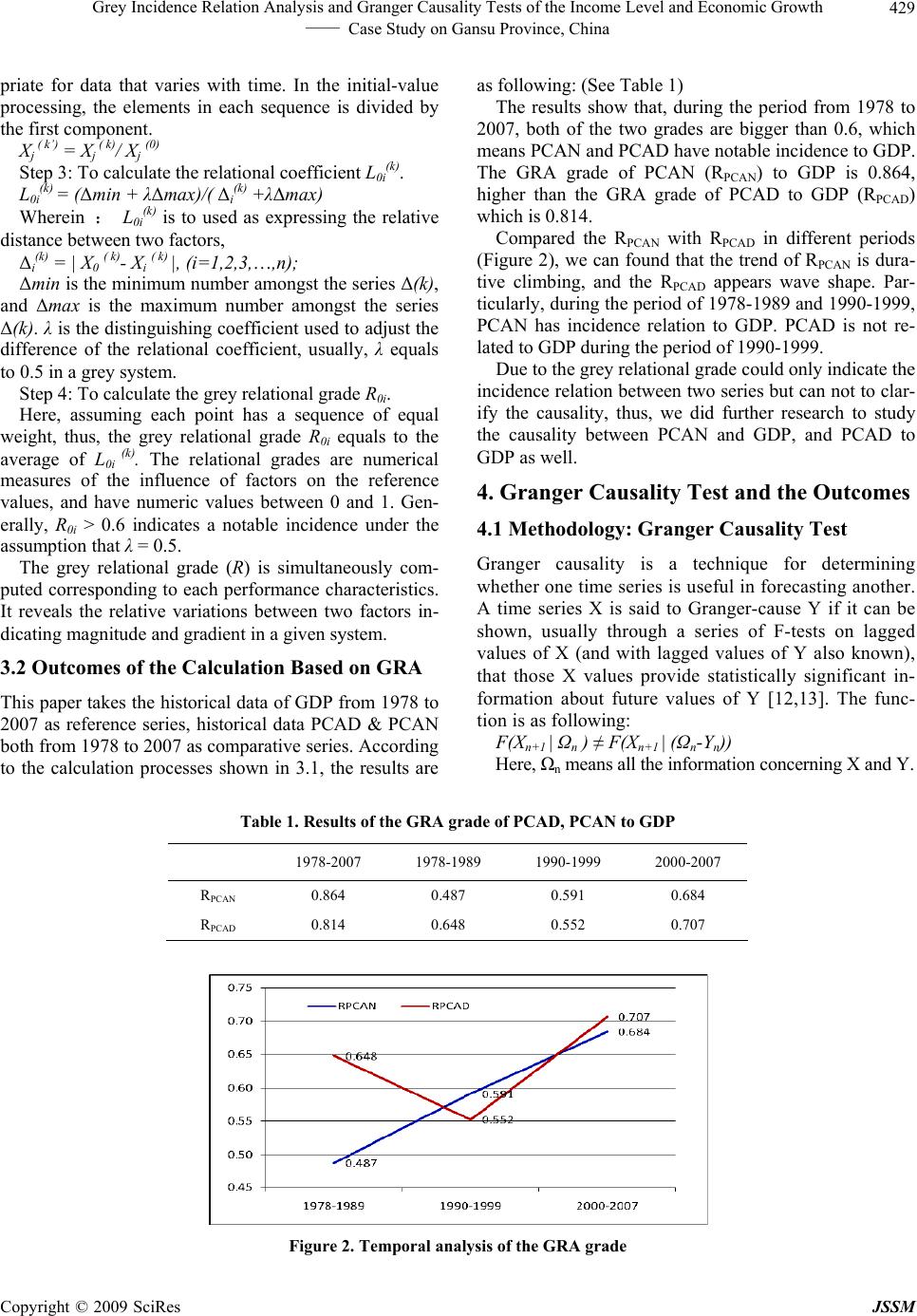 Grey Incidence Relation Analysis and Granger Causality Tests of the Income Level and Economic Growth 429 —— Case Study on Gansu Province, China priate for data that varies with time. In the initial-value processing, the elements in each sequence is divided by the first component. Xj ( k’) = Xj ( k)/ Xj (0) Step 3: To calculate the relational coefficient L0i (k). L0i (k) = (Δmin + λΔmax)/( Δi (k) +λΔmax) Wherein : L0i (k) is to used as expressing the relative distance between two factors, Δi (k) = | X0 ( k)- Xi ( k) |, (i=1,2,3,…,n); Δmin is the minimum number amongst the series Δ(k), and Δmax is the maximum number amongst the series Δ(k). λ is the distinguishing coefficient used to adjust the difference of the relational coefficient, usually, λ equals to 0.5 in a grey system. Step 4: To calculate the grey relational grade R0i. Here, assuming each point has a sequence of equal weight, thus, the grey relational grade R0i equals to the average of L0i (k). The relational grades are numerical measures of the influence of factors on the reference values, and have numeric values between 0 and 1. Gen- erally, R0i > 0.6 indicates a notable incidence under the assumption that λ = 0.5. The grey relational grade (R) is simultaneously com- puted corresponding to each performance characteristics. It reveals the relative variations between two factors in- dicating magnitude and gradient in a given system. 3.2 Outcomes of the Calculation Based on GRA This paper takes the historical data of GDP from 1978 to 2007 as reference series, historical data PCAD & PCAN both from 1978 to 2007 as comparative series. According to the calculation processes shown in 3.1, the results are as following: (See Table 1) The results show that, during the period from 1978 to 2007, both of the two grades are bigger than 0.6, which means PCAN and PCAD have notable incidence to GDP. The GRA grade of PCAN (RPCAN) to GDP is 0.864, higher than the GRA grade of PCAD to GDP (RPCAD) which is 0.814. Compared the RPCAN with RPCAD in different periods (Figure 2), we can found that the trend of RPCAN is dura- tive climbing, and the RPCAD appears wave shape. Par- ticularly, during the period of 1978-1989 and 1990-1999, PCAN has incidence relation to GDP. PCAD is not re- lated to GDP during the period of 1990-1999. Due to the grey relational grade could only indicate the incidence relation between two series but can not to clar- ify the causality, thus, we did further research to study the causality between PCAN and GDP, and PCAD to GDP as well. 4. Granger Causality Test and the Outcomes 4.1 Methodology: Granger Causality Test Granger causality is a technique for determining whether one time series is useful in forecasting another. A time series X is said to Granger-cause Y if it can be shown, usually through a series of F-tests on lagged values of X (and with lagged values of Y also known), that those X values provide statistically significant in- formation about future values of Y [12,13]. The func- tion is as following: F(Xn+1 | Ωn ) ≠ F(Xn+1 | (Ωn-Yn)) Here, Ωn means all the information concerning X and Y. Table 1. Results of the GRA grade of PCAD, PCAN to GDP 1978-2007 1978-1989 1990-1999 2000-2007 RPCAN 0.864 0.487 0.591 0.684 RPCAD 0.814 0.648 0.552 0.707 Figure 2. Temporal analysis of the GRA grade Copyright © 2009 SciRes JSSM  Grey Incidence Relation Analysis and Granger Causality Tests of the Income Level and Economic Growth 430 —— Case Study on Gansu Province, China Table 2. Causality tests of GDP to PCAN and PCAD Null Hypothesis L F-Sta. Prob. GDP does not Granger Cause PCAN 0.711 0.557 PCAN does not Granger Cause GDP 3 5.006 0.010 GDP does not Granger Cause PCAN 0.488 0.744 PCAN does not Granger Cause GDP 4 6.420 0.002 GDP does not Granger Cause PCAD 0.633 0.602 PCAD does not Granger Cause GDP 3 3.236 0.044 GDP does not Granger Cause PCAD 0.697 0.604 PCAD does not Granger Cause GDP 4 4.233 0.015 Table 3. Results of the generalized difference analysis Variables Coeff. Std. Err T-Sta Prob LNRURAL 0.7337 0.1043 7.0332 0.0000 LNURBAN 0.4817 0.0876 5.4978 0.0000 C -2.4008 0.3138 -7.6493 0.0000 AR(1) 1.1820 0.1960 6.0306 0.0000 AR(2) -0.4604 0.1976 -2.3300 0.0289 R-squared 0.9987 Mean dependent var 6.0219 Adjusted R2 0.9985 S.D. dependent var 1.1488 S.E. of regression 0.0452 Akaike info criterion -3.1942 Sum squared resid 0.0470 Schwarz criterion -2.9563 Log likelihood 49.7188 F-statistic 4350.749 DW stat 1.7002 Prob(F-statistic) 0.0000 4.2 Outcomes from the Tests Results Based on the software Eviews 3.2, we tested the causality. The results are in Table 2 below. The results show that, considering the notable lever equals to 10%, assuming the lags equals to 3 years or 4 years, under these scenarios, both the PCAN and PCAD are the Granger Cause GDP, which means there is sin- gle-causality between the two variables and GDP. In order to quantitative analyze the influence degree of the two variables and GDP; we use the Generalized Dif- ference Analysis to find out the influence degree by us- ing the software Eviews 3.2 under the program of Granger Causality Tests. See chapter 4.3 4.3 Generalized Difference Analysis and the Outcomes Before analyzing the differences, in order to remove the errors caused by the self-related series, we processed the series by taking the following change as following func- tion: X* = Xt – ρXt-1 The complete results are in following Table 3. The function of PCAD, PCAN, and GDP is: LNGDP = (-2.4008) + (0.7337* LNRURAL) + (0.4817* LNURBAN) Based on this function, we can find that, from 1978 to 2007, 1% unit increase of PCAN result in 0.7337% in- crease of GDP, but compared to PCAD, 1% unit increase of that only result in 0.4817% increase of GDP. 5. Conclusions This paper initiated to indicate the relationship between the economic growth and income level, and to find the scientific foundation to public policy making. The main conclusions are as following: GRA and GCT are appropriate methodologies to clar- ify the relation and grade. This research shows that the Copyright © 2009 SciRes JSSM  Grey Incidence Relation Analysis and Granger Causality Tests of the Income Level and Economic Growth 431 —— Case Study on Gansu Province, China GRA could be used to find out the incidence relation between the variables and the GCT is appropriate to test the causality and find out the influence degree. Hereby, based on the working progress when we studied the methodologies, we would like to point out seriously that the incidence relation does not equals to causality, which means, we cannot define the causality relation only ac- cording to the calculation results based on GRA. In the past years, the urban inhabitants shared the ma- jor outcomes due to the “Reform and Open” policy from 1978. On national level, averagely, per capita annual net income of rural households improved from 343.4 Yuan to 13,786 Yuan, instead, per capita annual net income of rural households improved from 133.6 Yuan to 4,140 Yuan, the gap between PCAN and PCAD in 2007 is 3.33 times. Nowadays, Chinese government released series of public policies with regard to improve the citizen income level, which aims to move forward the economic growth. This research indicates that to improve the rural house- hold’s income level is an urgent issue for China. The outcomes also proved that the national policy undertak- ing in the coming years of “improve the rural income and expand the domestic consumption” has scientific base and should be taken exactly in the next decade. REFERENCES [1] Z. G. Wen and J. N. Chen, “A cost-benefit analysis for the economic growth in China,” Ecological Economics, Vol. 65, pp. 356–366, 2008. [2] A. H. Carsten, “China’s economic growth 1978–2025: What we know today about china’s economic growth to- morrow,” World Development, Vol. 36, pp. 1665–1691, 2008. [3] World Bank, “China 2009 growth forecast to 6.5%,” China Quarterly Update, pp. 9, March 18, 2009. [4] R. Clarke, “More evidence on incomer distribution and growth [J],” Journal of Development Economics, Vol. 47, No. 2, pp. 403–427, 1995. [5] W. X. Zhou, “Case study of the relation between house- hold’s income and economic growth [J],” Economic Sci- ence, Vol. 1, pp. 40–47, 2002. [6] N. Zhao and Y. B. Wei, “Research on the income level and economic development,” Rural Economy, Science and Technology, Vol. 19, pp. 26–27, 2008. [7] E. Podrecca and G. Carmeci, “Fixed investment and eco- nomic growth: New results on causality,” Applied Eco- nomics, Vol. 33, pp. 177–182, 2001. [8] Y. Li and A. Oberheitmann, “Challenge of rapid eco- nomic growth in china: Reconciling sustainable energy use, environmental stewardship and social development,” Energy Policy, Vol. 37, pp. 1412–1422, 2009. [9] T. Persson and G. Tabellini, “Is inequality harmful for growth?” Theory and Evidence, American Economic Re- view, Vol. 84, pp. 600–621, 1994. [10] T. Persson and G. Tabellini, “Economic growth,” Quar- terly Journal of Economics, Vol. 77, pp. 465–490, 1994. [11] S. He, Y. Li, and R. Z. Wang, “A new approach to per- formance analysis of ejector refrigeration system using grey system theory,” Applied Thermal Engineering, Vol. 29, pp. 1592–1597, 2009. [12] G. X. Xu, “Statistic, forecast and decision making,” Shanghai: Shanghai Finance and Economy University Press, pp. 207, 2005. [13] Y. F. Cao, “Reviews on granger causality test,” World Economic Research, Vol. 2, pp. 16–21, 2005. Copyright © 2009 SciRes JSSM |