Vol.3, No.12, 999-1010 (2011) Natural Science
http://dx.doi.org/10.4236/ns.2011.312125
Analysis and comparison of spatial interpolation
methods for temperature data in Xinjiang Uygur
Autonomous Region, China
Huixia Chai1*, Weiming Cheng1, Chenghu Zhou1, Xi Chen2, Xiaoyi Ma1, Shangming Zhao2
1State Key Laboratory of Resources and Environmental Information System, Institute of Geographic Sciences and Natural Resources
Research CAS, Beijing, China; *Corresponding Author:
2Xinjiang Institute of Ecology and Geography CAS, Urumqi, China.
Received 24 October 2011; revised 20 November 2011; accepted 7 December 2011.
ABSTRACT
Spatial interpolation methods are frequently
used to estimate values of meteorological data
in locations where they are not measured.
However, very little research has been investi-
gated the relative performance of different in-
terpolation methods in meteorological data of
Xinjiang Uygur Autonomous Region (Xinjiang).
Actually, it has importantly practical signifi-
cance to as far as possibly improve the accu-
racy of interpolation results for meteorological
data, especially in mountainous Xinjiang. There-
fore, this paper focuses on the performance of
different spatial interpolation methods for
monthly temperature data in Xinjiang. The daily
observed data of temperature are collected from
38 meteorological stations for the period 1960-
2004. Inverse distance weighting (IDW), ordinary
kriging (OK), temperature lapse rate method
(TLR) and multiple linear regressions (MLR) are
selected as interpolated methods. Two raster-
ized methods, multiple regression plus space
residual error and directly interpolated ob-
served temperature (DIOT) data, are used to
analyze and compare the performance of these
interpolation methods respectively. Moreover,
cross-validation is used to evaluate the per-
formance of different spatial interpolation meth-
ods. The results are as follows: 1) The method
of DIOT is unsuitable for the study area in this
paper. 2) It is important to process the observed
data by local regression model before the spa-
tial interpolation. 3) The MLR-IDW is the opti-
mum spatial interpolation method for the monthly
mean temperature based on cross-validation.
For the authors, the reliability of results and the
influence of measurement accuracy, density, dis-
tribution and spatial variability on the accuracy
of the interpolation methods will be tested and
analyzed in the future.
Keywords: Spatial Interpolation Method; Cross
validation; Monthly Mean Temperature; Xinjiang
Uygur Autonomous Region
1. INTRODUCTION
Many researchers in different countries or various or-
ganizations from all over the world have put much effort
into interpolating the meteorological data [1-9]. Meas-
urements of meteorological data (e.g. temperature, hu-
midity, wind speed and rainfall) at higher resolution are
available only at limited stations because meteorological
data are generally recorded at specific locations and de-
rived from different meteorological stations. Moreover,
the essence of the spatial interpolation is to transfer
available information in the form of data from a number
of adjacent irregular sites to the estimated sites through a
function that represents the spatial weights according to
the distances between the sites [10]. For these reasons,
spatial interpolation methods are frequently used to es-
timate values of meteorological data in locations where
they are not measured [11].
Although a variety of deterministic and geo-statistical
interpolation methods are available to estimate variables
at un-sampled locations, accuracies vary widely among
methods [12]. The quality of climate spatial interpolation
depends on the spatial variation of climate factors, the
spatial distribution of climate stations, and the interpola-
tion method [13,14]. Consequently, many researchers try
to compare different spatial interpolation methods based
on different climate factors in various areas [15-19]. All
of these researches discussed various spatial interpola-
tion methods (including basic principle, application and

H. X. Chai et al. / Natural Science 3 (2011) 999-1010 1000
precision) of meteorological elements, valuable conclu-
sions were reached that the optimum spatial interpola-
tion method of one climate factor could not be suitable
for the other climate factors in the same area or the same
climate factor in different areas.
Actually, it is more difficult and important to build
climate layers as a result of sparse meteorological sta-
tions and complex topography [20]. Moreover, the opti-
mal spatial interpolation methods for various spatial
variables less appear and are applicable to the specific
conditions [21-25]. In different regions and various tem-
poral-spatial scales, the so-called “optimal” interpolation
is relatively. In other words, no one spatial interpolation
method is the absolutely optimal method due to the fea-
tures of interpolation method (e.g. hypothesis, tempo-
ral-spatial scale, algorithm, and attributes of data).
Xinjiang Uygur Autonomous Region is located in the
inner center of Eurasia. It is the core region of the arid
land in the northwest China. Xinjiang Uygur Autono-
mous Region has been one of the hot-spot areas in geo-
graphic research [26-34] due to its unique geomorpho-
logic features and important geographic location. How-
ever, only few researchers focused on seeking effective
methods of spatial interpolation for temperature [35-37]
and rainfall [38] in Xinjiang. Moreover, the conclusion
about the optimal method for temperature in Xinjiang is
different according to the research results of the above
mentioned literatures.
Therefore, the main objective of this paper is to find
out which one is the optimal interpolation method for
monthly mean temperature in Xinjiang Uygur Autono-
mous Region. Firstly, temperature data of Xinjiang from
many years are used to compare the performance of four
spatial interpolation methods, such as, Inverse distance
weighting, Ordinary kriging, Temperature lapse rate
method and Multiple linear regression with regard to
their errors by cross-validation. Secondly, two rasterized
methods (multiple regression plus space residual error,
direct interpolation with observed data of temperature)
are adopted to illustrate quality of spatial interpolation
methods. Finally, the conclusion as to which method is
significantly better than others on the basis of MBE,
MAE, and RMSE is proposed
2. METHOD AND MATERIAL
2.1. Study Area
The study area of this research is Xinjiang Uygur
Autonomous Region, lying in the middle of Asia’s con-
tinental shelf. It is located between 34˚ ~ 50˚N, 75˚ ~
97˚E, northwest of China (Figure 1). The Xinjiang’s
climate is mainly controlled by three factors: geographi-
cal location (far away from the ocean), terrain structure
(mountain and basin) and the Qinghai-Tibet Plateau
[39].
The basic geomorphologic pattern of Xinjiang in and
abroad is the direct cause of local climate. The Himalayas
Figure 1. Study area and the distribution of meteorological stations.

H. X. Chai et al. / Natural Science 3 (2011) 999-1010
1001001
and Qinghai-Tibet Plateau block the southwest monsoon
from the Indian Ocean with rich content of water vapor.
The southeast monsoon from Pacific Ocean has little
chance to reach Xinjiang, because it is obstructed by
circumambient mountains such as Qinling Mountains,
Greater Hinggan Mountains, Qilian Mountain, and Qing-
hai-Tibet Plateau. The north air current from Arctic
Ocean usually pass through Altay Mountains and can
arrive in Xinjiang. But it mainly distributes in the north
of Xinjiang. Moreover, it can form less rainfall because
the air current from Arctic Ocean belongs to dry and
cold air with poor content of water. Temperature of
southern Xinjiang is higher than that of northern Xinji-
ang. According to the latitude zones, southern Xinjiang
and northern Xinjiang belong to warm temperate zone
and temperate zone respectively. The zone differentia-
tion becomes enhancement due to the blocking of Tian-
shan Mountains. The annual frost-free period is about
200 - 220 days in plain area of southern Xinjiang, how-
ever, it is about 150 days in northern Xinjiang [39].
2.2. Data
The main data source of this paper includes meteoro-
logical data and SRTM-DEM.
In this article, daily observed data are collected from
54 meteorological stations in Xinjiang during the period
1951-2009. These meteorological stations are both Na-
tional basic stations and province benchmark stations. In
all, 38 meteorological stations for the period 1960-2004
are picked out after analyzing and quality control pro-
cedure based on Microsoft Office Access and Geo-
graphic information system (GIS). The distribution of 38
meteorological stations is showed in the Figure 1.
The Shuttle Radar Topography Mission digital eleva-
tion model (SRTM-DEM) (USGS, 2004) is used to ex-
tract the elevation value in this article. The resolution of
SRTM-DEM data is 90 × 90 m.
2.3. Methodology
In recent years, some researchers developed many
modified interpolation methods [10,13,35,40]. Based on
the rasterized method of temperature data, most re-
searches show that method of “multiple regression plus
space residual error” is better than that of “directly in-
terpolated for observe data of temperature” [36,37,41].
For the study area, IDW, Ordinary Kriging (OK), Tem-
perature lapse rate method (TLR), and Multiple linear
regression (MLR) are selected in this article to compare
their performance for monthly mean temperature. IDW
and OK are used to directly interpolate observed data of
temperature. TLR and MLR are used to interpolate revi-
sionary data. That means observed data should be re-
vised by regression formula before interpolating. The
following is briefly introduction of interpolation meth-
ods used in this study.
1) Inverse Distance Weighting. The IDM value is
given by the following formula.
 
38
0
1
ii
i
Ts Ts 

 (1)
In Formula 1,


0
Ts is predicted value of 0
s
(pre-
dicted point), i

is power coefficient of sampled points,


i
Ts is observed value of i
s
(sampled point).
2) Ordinary Kriging. The method is expressed as fol-
lowing formula.
 
0
1
n
ii
i
Z
sZs 

 (2)
In the Formula 2, the weight is derived from the
Kriging system in following formula (i = 1, 2, , n).


0
1
1
1
n
iij i
i
n
i
i
s
sss  



 








(3)
3) Temperature lapse rate method (TLR) can use fol-
lowing formulate.
100
100
so o
es d
TTbH
TTbH



 (No elevation error) (4)
100
100
so d
es d
TTbH
TTbH





 (With elevation error) (5)
ee
TTT


 (6)
In Formula 4, Formula 5 and Formula 6,


s
s
TT

is
revisionary temperature of the virtual sea level (˚C), o
T
is observed temperature of meteorological station (˚C), b
is temperature lapse rate,

ee
TT
 is estimated tempera-
ture (˚C), o
H
is observed elevation of meteorological
station (m), d
H
is elevation value from DEM of point
which has the same coordinates with that of meteoro-
logical station (m), T

is difference between e T and
e
T

(˚C).
4) Multiple Linear Regression (MLR). Firstly, regres-
sion formula with elevation, latitude, and longitude is
built.
TaHbLacLoE


(7)
In Formula 7, T is temperature, a, b, c are regression
coefficients, H is elevation, La is latitude, Lo is longi-
tude, E is residual error. Least-square method is used to
obtain parameters, such as a, b, c, E. The equations set
are expressed as follows.

H. X. Chai et al. / Natural Science 3 (2011) 999-1010 1002
2
2
2
TnEaHbLacLo
THE HaHbHbHLacHLo
TLaELaaHLa bLacLaLo
TLo ELoaHLobLaLocLo
 

 

 

 




 
(8)
The following matrix is used to obtain parameters
value.

1
Bxx xy



(9)
E
a
Bb
c






,

2
2
2
nHLaLo
H
HHLaHLo
xx La HLaLaLaLo
Lo HLo LaLoLo







 
 

 
,

T
TH
xy TLa
TLo











Secondly, Eq.7 and SRTM-DEM are used to estimate
the temperature of study area. The output data is named
estimated temperature (ˆ
e
T).
Thirdly, interpolation residual error E is analyzed. The
interpolation method includes IDW and OK. The output
data is named residual error layer.
Finally, the estimated temperature (ˆ
ee
TTE) is
gained through overlaying two data layers, that is, esti-
mated temperature and residual error layer.
The most common one for assessing prediction errors
of spatial interpolation methods is cross-validation. Gen-
erally, the mean/mean-biased error (ME or MBE), the
mean absolute error (MAE), and the root mean squared
error (RMSE) are used to estimate the error statistic.
Other researchists use standardized RMSE as an addi-
tional measure to evaluate the uncertainty of Kriging
statistics [11,42]. Consequently, cross-validation is used
to evaluate the performance of different spatial interpo-
lation methods in this paper. To describe the perform-
ance of interpolation methods, the deviations of valida-
tion results are summarized by three average error statis-
tics methods, such as, RMSE, MAE and MBE (ME).
2.4. Computational Details
Spatial analyst tool and geostatistical analyst tool of
ArcGIS are used to interpolate and analyze temperature
data in this paper.
Based on ArcGIS, the function of IDW has two op-
tions, that is, a fixed search radius type and a variable
search radius type. In this study, the variable radius type
is selected because sample points are sparse and ran-
domly placed.
For Kriging method, cross validation techniques are
used to choose spherical semivariogram model because
it (spherical model) is widely used. In this search, radius
is used as variable with default value.
To decide whether the model can be applied, it is
necessary to verify and estimate multiple linear regres-
sion model after obtaining the regression parameters.
The content and method for testing and estimating in-
clude fitting degree test (R-squared, R2), standard devia-
tion test (ST), and significance test (F).
3. RESULTS AND DISCUSSION
3.1. Meteorological Data
The quality control procedure can ensure the continu-
ity and effectiveness of data in our research. Daily ob-
served data of temperature is collected from 54 mete-
orological stations for the period 1951-2009. After ana-
lyzing quality of meteorological data, 29.62% of stations
are rejected because of missing data or short duration,
11.06% of the observed data is filtered out because of
invalid data or unreasonable temporal sequence. The
monthly mean temperature values of 38 meteorological
stations area selected for the period 1960-2004.
Therefore, the number of stations is rare for the study
area and their distribution is inordinate because of com-
plex topography (Figure 1). Most stations locate in plain
area. Few stations distribute in the intermountain basin
of Tianshan Mountains. Other mountain areas have no
stations. However, temperature in mountainous region
decreases with the increasing of altitude. Moreover, de-
serts in the basin will affect temperature in plain area.
Consequently, there exists the possible error between the
interpolation result and observed temperature.
According to Figure 2, the minimum temperature ap-
pears in No. 22 of all meteorological stations in every
month, and the highest temperature distributes in No. 24.
This means the temperature of Yourdus Basin, located in
middle Tianshan Mountains, is the lowest per month.
Moreover, the temperature of Turpan Basin is the high-
est (Figure 1).
Table 1 shows the values of average, maximum, and
minimum of monthly mean temperature for the period
1960-2004 in study area. According to the Table 1, the
highest value of the maximum temperature is 32.39˚C in
July. The lowest value of the maximum temperature is

H. X. Chai et al. / Natural Science 3 (2011) 999-1010
1001003
Figure 2. The line chart of monthly mean temperature.
Table 1. Monthly mean temperatures for the period 1960-2004
(˚C).
Month 1 2 3 4 5 6
Tmax –4.51 0.48 9.75 19.08 26.0531.08
Tmin –26.46 –22.31 –10.92 0.34 5.51 8.90
Taverage –11.71 –7.51 1.76 11.36 17.78 22.22
Month 7 8 9 10 11 12
Tmax 32.39 30.21 23.2513.06 4.37 –2.87
Tmin 10.71 9.91 5.60 –1.81 –11.54–21.34
Taverage 23.63 22.31 16.65 8.23 –0.94–8.95
–4.51˚C in January. For the minimum temperature of
monthly mean temperature, the maximum value is
10.71˚C in July and the minimum value is –26.46˚C in
January.
According the data sets, July is the hottest month and
January is the coldest month. Therefore, monthly mean
temperature of June, July and August is selected to stand
for summer temperature, and monthly mean temperature
of December, January and February to represent winter
temperature in this study.
3.2. Comparison of Interpolation Methods
Spatial interpolation is an extremely important method
for the spatial analysis of GIS. For a region with scarce
and unreasonable distribution of observation stations,
spatial interpolation is the basic method for studying the
distribution of spatial variables. This is one of the prem-
ises to establish spatial model. Three ways are used to
examine the performance of the interpolation methods
above mentioned in this paper.
3.2.1. Directly Interpolating Observed
Temperature (DIOT)
This section analyzes the performance of IDW and
OK. These two methods are applied to interpolate the
observed temperature directly.
According to Table 2, it is not a good idea to interpo-
late observed temperature directly for this study area.
Obviously, the RMSE values of validation results by
DIOT are too big.
The error values of calculation on the basis of the
validation result (Table 2), both IDW and OK, are too
big. Consequently, it is not a good idea to interpolate the
observed temperature data directly for Xinjiang. In other
words, it is necessary to revise the observed data before
implementing spatial interpolation.
3.2.2. Temperature Lapse Rate Method (TLR)
3.2.2.1. Difference of Elevation
TLR considers temperature will decrease with the in-
crease of altitude. Table 3 shows the difference between
elevation based on meteorological stations and elevation
from corresponding SRTM-DEM. The biggest differ-
ence of elevation can reach up to 103.7 m. The smallest
difference of elevation is 0.2 m. Moreover, the elevation
differences of most stations are less than 10 m.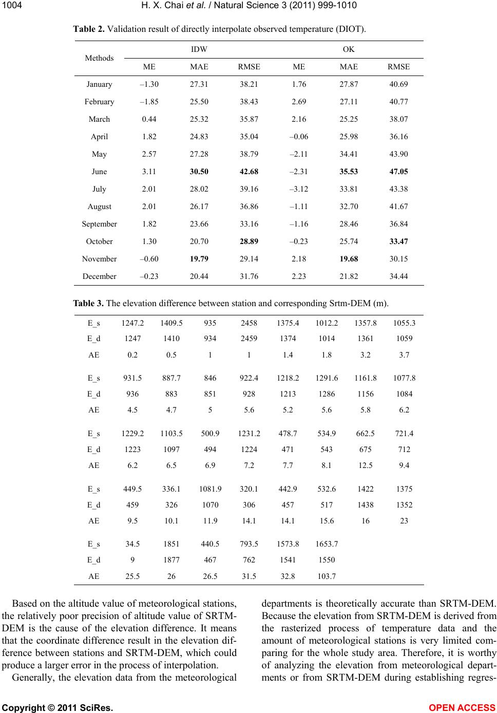

H. X. Chai et al. / Natural Science 3 (2011) 999-1010 1004
Table 2. Validation result of directly interpolate observed temperature (DIOT).
IDW OK
Methods
ME MAE RMSE ME MAE RMSE
January –1.30 27.31 38.21 1.76 27.87 40.69
February –1.85 25.50 38.43 2.69 27.11 40.77
March 0.44 25.32 35.87 2.16 25.25 38.07
April 1.82 24.83 35.04 –0.06 25.98 36.16
May 2.57 27.28 38.79 –2.11 34.41 43.90
June 3.11
30.50 42.68 –2.31 35.53 47.05
July 2.01 28.02 39.16 –3.12 33.81 43.38
August 2.01 26.17 36.86 –1.11 32.70 41.67
September 1.82 23.66 33.16 –1.16 28.46 36.84
October 1.30 20.70 28.89 –0.23 25.74 33.47
November –0.60 19.79 29.14 2.18 19.68 30.15
December –0.23 20.44 31.76 2.23 21.82 34.44
Table 3. The elevation difference between station and corresponding Srtm-DEM (m).
E_s 1247.2 1409.5 935 2458 1375.4 1012.2 1357.8 1055.3
E_d 1247 1410 934 2459 1374 1014 1361 1059
AE 0.2 0.5 1 1 1.4 1.8 3.2 3.7
E_s 931.5 887.7 846 922.4 1218.2 1291.6 1161.8 1077.8
E_d 936 883 851 928 1213 1286 1156 1084
AE 4.5 4.7 5 5.6 5.2 5.6 5.8 6.2
E_s 1229.2 1103.5 500.9 1231.2 478.7 534.9 662.5 721.4
E_d 1223 1097 494 1224 471 543 675 712
AE 6.2 6.5 6.9 7.2 7.7 8.1 12.5 9.4
E_s 449.5 336.1 1081.9 320.1 442.9 532.6 1422 1375
E_d 459 326 1070 306 457 517 1438 1352
AE 9.5 10.1 11.9 14.1 14.1 15.6 16 23
E_s 34.5 1851 440.5 793.5 1573.8 1653.7
E_d 9 1877 467 762 1541 1550
AE 25.5 26 26.5 31.5 32.8 103.7
Based on the altitude value of meteorological stations,
the relatively poor precision of altitude value of SRTM-
DEM is the cause of the elevation difference. It means
that the coordinate difference result in the elevation dif-
ference between stations and SRTM-DEM, which could
produce a larger error in the process of interpolation.
Generally, the elevation data from the meteorological
departments is theoretically accurate than SRTM-DEM.
Because the elevation from SRTM-DEM is derived from
the rasterized process of temperature data and the
amount of meteorological stations is very limited com-
paring for the whole study area. Therefore, it is worthy
of analyzing the elevation from meteorological depart-
ments or from SRTM-DEM during establishing regres-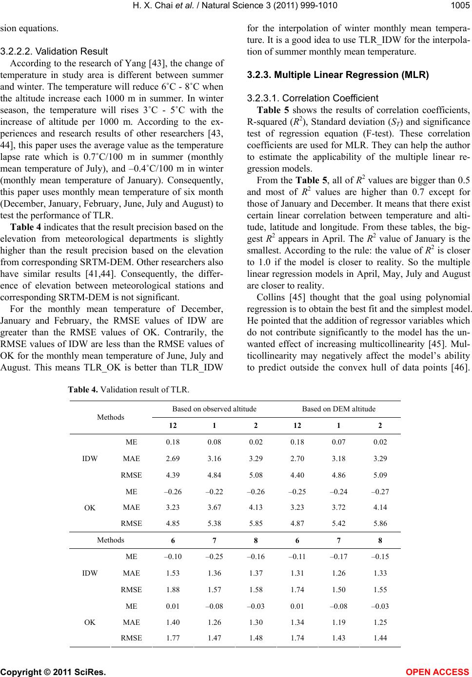

H. X. Chai et al. / Natural Science 3 (2011) 999-1010
1001005
sion equations.
3.2.2.2. Validation Result
According to the research of Yang [43], the change of
temperature in study area is different between summer
and winter. The temperature will reduce 6˚C - 8˚C when
the altitude increase each 1000 m in summer. In winter
season, the temperature will rises 3˚C - 5˚C with the
increase of altitude per 1000 m. According to the ex-
periences and research results of other researchers [43,
44], this paper uses the average value as the temperature
lapse rate which is 0.7˚C/100 m in summer (monthly
mean temperature of July), and –0.4˚C/100 m in winter
(monthly mean temperature of January). Consequently,
this paper uses monthly mean temperature of six month
(December, January, February, June, July and August) to
test the performance of TLR.
Table 4 indicates that the result precision based on the
elevation from meteorological departments is slightly
higher than the result precision based on the elevation
from corresponding SRTM-DEM. Other researchers also
have similar results [41,44]. Consequently, the differ-
ence of elevation between meteorological stations and
corresponding SRTM-DEM is not significant.
For the monthly mean temperature of December,
January and February, the RMSE values of IDW are
greater than the RMSE values of OK. Contrarily, the
RMSE values of IDW are less than the RMSE values of
OK for the monthly mean temperature of June, July and
August. This means TLR_OK is better than TLR_IDW
for the interpolation of winter monthly mean tempera-
ture. It is a good idea to use TLR_IDW for the interpola-
tion of summer monthly mean temperature.
3.2.3. Multiple Linear Regression (MLR)
3.2.3.1. Correlation Coefficient
Table 5 shows the results of correlation coefficients,
R-squared (R2), Standard deviation (ST) and significance
test of regression equation (F-test). These correlation
coefficients are used for MLR. They can help the author
to estimate the applicability of the multiple linear re-
gression models.
From the Table 5, all of R2 values are bigger than 0.5
and most of R2 values are higher than 0.7 except for
those of January and December. It means that there exist
certain linear correlation between temperature and alti-
tude, latitude and longitude. From these tables, the big-
gest R2 appears in April. The R2 value of January is the
smallest. According to the rule: the value of R2 is closer
to 1.0 if the model is closer to reality. So the multiple
linear regression models in April, May, July and August
are closer to reality.
Collins [45] thought that the goal using polynomial
regression is to obtain the best fit and the simplest model.
He pointed that the addition of regressor variables which
do not contribute significantly to the model has the un-
wanted effect of increasing multicollinearity [45]. Mul-
ticollinearity may negatively affect the model’s ability
to predict outside the convex hull of data points [46].
Table 4. Validation result of TLR.
Based on observed altitude Based on DEM altitude
Methods
12 1 2 12 1 2
ME 0.18 0.08 0.02 0.18 0.07 0.02
MAE 2.69 3.16 3.29 2.70 3.18 3.29 IDW
RMSE 4.39 4.84 5.08 4.40 4.86 5.09
ME –0.26 –0.22 –0.26 –0.25 –0.24 –0.27
MAE 3.23 3.67 4.13 3.23 3.72 4.14 OK
RMSE 4.85 5.38 5.85 4.87 5.42 5.86
Methods 6 7 8 6 7 8
ME –0.10 –0.25 –0.16 –0.11 –0.17 –0.15
MAE 1.53 1.36 1.37 1.31 1.26 1.33 IDW
RMSE 1.88 1.57 1.58 1.74 1.50 1.55
ME 0.01 –0.08 –0.03 0.01 –0.08 –0.03
MAE 1.40 1.26 1.30 1.34 1.19 1.25 OK
RMSE 1.77 1.47 1.48 1.74 1.43 1.44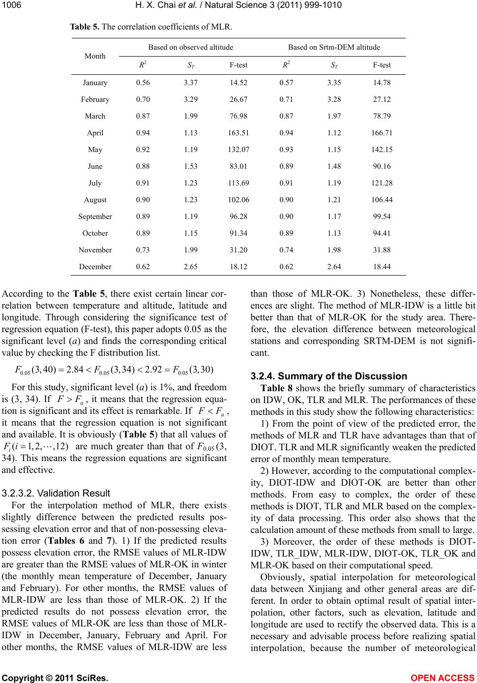

H. X. Chai et al. / Natural Science 3 (2011) 999-1010 1006
Table 5. The correlation coefficients of MLR.
Based on observed altitude Based on Srtm-DEM altitude
Month
R2 ST F-test R2 ST F-test
January 0.56 3.37 14.52 0.57 3.35 14.78
February 0.70 3.29 26.67 0.71 3.28 27.12
March 0.87 1.99 76.98 0.87 1.97 78.79
April 0.94 1.13 163.51 0.94 1.12 166.71
May 0.92 1.19 132.07 0.93 1.15 142.15
June 0.88 1.53 83.01 0.89 1.48 90.16
July 0.91 1.23 113.69 0.91 1.19 121.28
August 0.90 1.23 102.06 0.90 1.21 106.44
September 0.89 1.19 96.28 0.90 1.17 99.54
October 0.89 1.15 91.34 0.89 1.13 94.41
November 0.73 1.99 31.20 0.74 1.98 31.88
December 0.62 2.65 18.12 0.62 2.64 18.44
According to the Table 5, there exist certain linear cor-
relation between temperature and altitude, latitude and
longitude. Through considering the significance test of
regression equation (F-test), this paper adopts 0.05 as the
significant level (a) and finds the corresponding critical
value by checking the F distribution list.
0.050.05 0.05
(3, 40)2.84(3,34)2.92(3,30)FFF
For this study, significant level (a) is 1%, and freedom
is (3, 34). If a
F
F, it means that the regression equa-
tion is significant and its effect is remarkable. If a
F
F

,
it means that the regression equation is not significant
and available. It is obviously (Table 5) that all values of
(1,2,,12)
i
Fi are much greater than that of F0.05 (3,
34). This means the regression equations are significant
and effective.
3.2.3.2. Validation Result
For the interpolation method of MLR, there exists
slightly difference between the predicted results pos-
sessing elevation error and that of non-possessing eleva-
tion error (Tables 6 and 7). 1) If the predicted results
possess elevation error, the RMSE values of MLR-IDW
are greater than the RMSE values of MLR-OK in winter
(the monthly mean temperature of December, January
and February). For other months, the RMSE values of
MLR-IDW are less than those of MLR-OK. 2) If the
predicted results do not possess elevation error, the
RMSE values of MLR-OK are less than those of MLR-
IDW in December, January, February and April. For
other months, the RMSE values of MLR-IDW are less
than those of MLR-OK. 3) Nonetheless, these differ-
ences are slight. The method of MLR-IDW is a little bit
better than that of MLR-OK for the study area. There-
fore, the elevation difference between meteorological
stations and corresponding SRTM-DEM is not signifi-
cant.
3.2.4. Summary of the Discussion
Table 8 shows the briefly summary of characteristics
on IDW, OK, TLR and MLR. The performances of these
methods in this study show the following characteristics:
1) From the point of view of the predicted error, the
methods of MLR and TLR have advantages than that of
DIOT. TLR and MLR significantly weaken the predicted
error of monthly mean temperature.
2) However, according to the computational complex-
ity, DIOT-IDW and DIOT-OK are better than other
methods. From easy to complex, the order of these
methods is DIOT, TLR and MLR based on the complex-
ity of data processing. This order also shows that the
calculation amount of these methods from small to large.
3) Moreover, the order of these methods is DIOT-
IDW, TLR_IDW, MLR-IDW, DIOT-OK, TLR_OK and
MLR-OK based on their computational speed.
Obviously, spatial interpolation for meteorological
data between Xinjiang and other general areas are dif-
ferent. In order to obtain optimal result of spatial inter-
polation, other factors, such as elevation, latitude and
longitude are used to rectify the observed data. This is a
necessary and advisable process before realizing spatial
interpolation, because the number of meteorological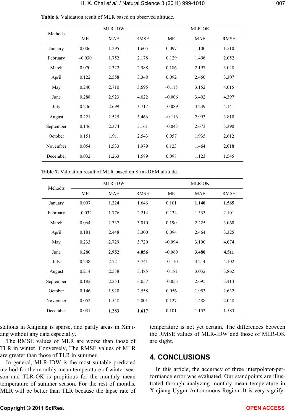

H. X. Chai et al. / Natural Science 3 (2011) 999-1010
1001007
Table 6. Validation result of MLR based on observed altitude.
MLR-IDW MLR-OK
Methods
ME MAE RMSE ME MAE RMSE
January 0.006 1.295 1.605 0.097 1.100 1.510
February –0.030 1.752 2.178 0.129 1.496 2.052
March 0.070 2.322 2.988 0.186 2.197 3.028
April 0.122 2.558 3.348 0.092 2.450 3.307
May 0.240 2.710 3.695 –0.115 3.152 4.015
June 0.288 2.923 4.022 –0.006 3.402 4.397
July 0.246 2.699 3.717 –0.089 3.239 4.141
August 0.221 2.525 3.466 –0.116 2.993 3.810
September 0.146 2.374 3.161 –0.043 2.673 3.390
October 0.151 1.911 2.543 0.057 1.935 2.612
November 0.054 1.533 1.979 0.123 1.464 2.018
December 0.032 1.263 1.589 0.098 1.123 1.545
Table 7. Validation result of MLR based on Srtm-DEM altitude.
MLR-IDW MLR-OK
Mehodts
ME MAE RMSE ME MAE RMSE
January 0.007 1.324 1.646 0.101 1.140 1.565
February –0.032 1.776 2.214 0.134 1.533 2.101
March 0.064 2.337 3.010 0.190 2.225 3.060
April 0.181 2.448 3.300 0.094 2.464 3.325
May 0.233 2.729 3.720 –0.094 3.190 4.074
June 0.280 2.952 4.056 –0.069 3.480 4.511
July 0.238 2.721 3.741 –0.110 3.214 4.102
August 0.214 2.538 3.485 –0.181 3.032 3.862
September 0.182 2.254 3.057 –0.053 2.695 3.414
October 0.146 1.920 2.558 0.056 1.953 2.632
November 0.052 1.548 2.001 0.127 1.488 2.048
December 0.031 1.283 1.617 0.101 1.152 1.583
stations in Xinjiang is sparse, and partly areas in Xinji-
ang without any data especially.
The RMSE values of MLR are worse than those of
TLR in winter. Conversely, The RMSE values of MLR
are greater than those of TLR in summer.
In general, MLR-IDW is the most suitable predicted
method for the monthly mean temperature of winter sea-
son and TLR-OK is propitious for the monthly mean
temperature of summer season. For the rest of months,
MLR will be better than TLR because the lapse rate of
temperature is not yet certain. The differences between
the RMSE values of MLR-IDW and those of MLR-OK
are slight.
4. CONCLUSIONS
In this article, the accuracy of three interpolator-per-
formance error was evaluated. Our standpoints are illus-
trated through analyzing monthly mean temperature in
Xinjiang Uygur Autonomous Region. It is very signify-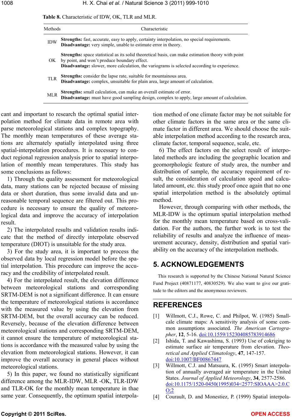

H. X. Chai et al. / Natural Science 3 (2011) 999-1010 1008
Table 8. Characteristic of IDW, OK, TLR and MLR.
Methods Characteristic
IDW Strengths: fast, accurate, easy to apply, certainty interpolation, no special requirements.
Disadvantage: very simple, unable to estimate error in theory.
OK
Strengths: space statistical as its solid theoretical basis, can make estimation theory with point
by point, and won’t produce boundary effect.
Disadvantage: slower, more calculation, the variograms is selected according to experience.
TLR Strengths: consider the lapse rate, suitable for mountainous area.
Disadvantage: complex, unsuitable for plain area, large amount of calculation.
MLR Strengths: small calculation, can make an overall estimate of error.
Disadvantage: must have good sampling design, complex to apply, large amount of calculation.
cant and important to research the optimal spatial inter-
polation method for climate data in remote area with
parse meteorological stations and complex topography.
The monthly mean temperatures of these average sta-
tions are alternately spatially interpolated using three
spatial-interpolation procedures. It is necessary to con-
duct regional regression analysis prior to spatial interpo-
lation of monthly mean temperatures. This study has
some conclusions as follows:
1) Through the quality assessment for meteorological
data, many stations can be rejected because of missing
data or short duration, thus some invalid data and un-
reasonable temporal sequence are filtered out. This pro-
cedure is necessary to ensure the quality of meteoro-
logical data and improve the accuracy of interpolation
result.
2) The interpolated results and validation results indi-
cate that the method of directly interpolate observed
temperature (DIOT) is unsuitable for the study area.
3) For the study area, it is important to process the
observed data by local regression model before the spa-
tial interpolation. This procedure can improve the accu-
racy and the credibility of interpolated result.
4) For the interpolated result, the elevation difference
between meteorological stations and corresponding
SRTM-DEM is not a significant difference. It can ensure
the temperature of meteorological stations is accordance
with the measured value by using the elevation from
SRTM-DEM, but the overall accuracy can be reduced.
Reversely, because of the elevation difference between
meteorological stations and corresponding SRTM-DEM,
it cannot ensure the temperature of meteorological sta-
tions is accordance with the measured value by using the
elevation from meteorological stations. However, it can
improve the overall accuracy in general places without
meteorological stations.
5) In this paper, we found no statistically significant
difference among the MLR-IDW, MLR -OK, TLR-IDW
and TLR-OK for the monthly mean temperature in thae
same year. Consequently, the optimum spatial interpola-
tion method of one climate factor may be not suitable for
other climate factors in the same area or the same cli-
mate factor in different area. We should choose the suit-
able interpolation method according to the research area,
climate factor, temporal sequence, scale, etc.
6) The effect factors on the select result of interpo-
lated methods are including the geographic location and
geomorphologic feature of study area, the number and
distribution of sample, the accuracy requirement of re-
sult, the consideration of calculation speed and calcu-
lated amount, etc. this study proof once again that no one
spatial interpolation method is the absolutely optimal
method.
However, through comparing with other methods, the
MLR-IDW is the optimum spatial interpolation method
for the monthly mean temperature based on cross-vali-
dation. For the authors, the further work is to test the
reliability of results and analyze the influence of meas-
urement accuracy, density, distribution and spatial vari-
ability on the accuracy of the interpolation methods.
5. ACKNOWLEDGEMENTS
This research is supported by the Chinese National Natural Science
Fund Project (40871177, 40830529). We also want to give our grati-
tude to the editors and the anonymous reviewers.
REFERENCES
[1] Willmott, C.J., Rowe, C. and Philpot, W. (1985) Small-
cale climate maps: A sensitivity analysis of some com-
mon assumptions associated. The American Cartogra-
pher, 12, 5-16. doi:10.1559/152304085783914686
[2] Ishida, T. and Kawashima, S. (1993) Use of cokriging to
estimate surface air temperature from elevation. Theo-
retical and Applied Climatology, 47, 147-157.
doi:10.1007/BF00867447
[3] Willmott, C.J. and Matsuura, K. (1995) Smart interpola-
tion of annually averaged air temperature in the United
States. Journal of Applied Meteorology, 34, 2577-2586.
doi:10.1175/1520-0450(1995)034<2577:SIOAAA>2.0.C
O;2
[4] Courault, D. and Monestiez, P. (1999) Spatial interpola-

H. X. Chai et al. / Natural Science 3 (2011) 999-1010
1001009
tion of air temperature according to atmospheric circula-
tion patterns in southeast France. International Journal
of Climatology, 19, 365-378.
doi:10.1002/(SICI)1097-0088(19990330)19:4<365::AID
-JOC369>3.0.CO;2-E
[5] Price, D.T., McKenney, D.W., Nalder, I.A., Hutchinson,
M. F. and Kesteven, J.L. (2000) A comparison of two sta-
tistical methods for spatial interpolation of Canadian
monthly mean climate data. Agricultural and Forest Me-
teorology, 101, 81-94.
doi:10.1016/S0168-1923(99)00169-0
[6] Hofierka, J., Parajka, J., Mitasova, H. and Mitas, L.
(2002) Multivariate interpolation of precipitation using
regularized spline with tension. Transactions in GIS, 6,
135-150. d oi :1 0. 1111/1467-9671.00101
[7] Rawlins, M.A. and Willmott, C.J. (2003) Winter air tem-
perature change over the terrestrial arctic, 1961-1990.
Arctic, Antarctic, and Alpine Research, 35, 530-537.
doi:10.1657/1523-0430(2003)035[0530:WATCOT]2.0.C
O;2
[8] Dobesch, H., Dumolard, P. and Dyras, I. (2007) Spatial
interpolation for climate data: The use of GIS in clima-
tology and meteorology. ISTE Ltd., London.
[9] Muhammad, W.A., Zhao, C., Ni, J. and Muhammad, A.
(2010) GIS-based high-resolution spatial interpolation of
precipitation in mountain-plain areas of Upper Pakistan
for regional climate change impact studies. Theoretical
and Applied Climatology, 99, 239-253.
doi:10.1007/s00704-009-0140-y
[10] Şen, Z. and Şahin, A. D. (2001) Spatial interpolation and
estimation of solar irradiation by cumulative semivario-
grams. Solar Energy, 71, 11-21.
doi:10.1016/S0038-092X(01)00009-3
[11] Murphy, R.R., Curriero, F.C., Ball, W.P. and Asce, M.
(2010) Comparison of spatial interpolation methods for
water quality evaluation in the chesapeake bay. Journal
of Environmental Engineering, 136, 160-171.
doi:10.1061/(ASCE)EE.1943-7870.0000121
[12] Luo, W., Taylor, M.C. and Parker, S.R. (2008) A com-
parison of spatial interpolation methods to estimate con-
tinuous wind speed surfaces using irregularly distributed
data from England and Wales. International Journal of
Climatology, 28, 947-99. doi:10.1002/joc.1583
[13] Janis, M.J., Hubbard, K.G. and Redmond, K.T. (2004)
Station density strategy for monitoring long term climatic
change in the contiguous United States. Journal of cli-
mate, 17, 151-162.
doi:10.1175/1520-0442(2004)017<0151:SDSFML>2.0.C
O;2
[14] Kong, Y. and Tong, W. (2008) Spatial exploration and
interpolation of the surface precipitation data. Geo-
graphical Research, 27, 1097-1108 (in Chinese).
[15] Abtew, W., Obeysekera, J. and Shih, G. (1993) Spatial
analysis for monthly rainfall in South Florida. Water Re-
sources Bulletin.American Water Resources Association,
29, 179-188. doi :1 0. 1111/ j.1752-1688.1993.tb03199.x
[16] Anderson, S. (2002) An evaluation of spatial interpola-
tion methods on air temperature in Phoenix, AZ. De-
partment of Geography, Arizona State University.
http://www.cobblestoneconcepts.com/ucgis2summer/and
erson/anderson.htm
[17] Daly, C., Helmer, E.H. and Quiñones, M. (2003) Map-
ping the climate of Puerto Rico, Vieques and Culebra.
International Journal of Climatology, 23, 1359-1381.
doi:10.1002/joc.937
[18] Zhu, H., Liu, S. and Jia, S. (2004) Problems of the spatial
interpolation of physical geographical elements. Geo-
graphical Research, 23, 425-432. (in Chinese)
[19] Li, M., Shao, Q. and Renzullo, L. (2010) Estimation and
spatial interpolation of rainfall intensity distribution from
the effective rate of precipitation. Stoch Environ Res Risk
Assess, 24, 117-130. doi:10.1007/s00477-009-0305-3
[20] Chiu, C., Lin, P. and Lu, K. (2009). GIS-based tests for
quality control of meteorological data and spatial inter-
polation of climate data—A case study in mountainous
Taiwan. Mountain Research and Development, 29, 339-
49. doi:10.1659/mrd.00030
[21] Dodson, R. and Marks, D. (1997) Daily air temperature
interpolated at high spatial resolution over a large moun-
tainous region. Climate Resource, 8, 1-20.
doi:10.3354/cr008001
[22] Dubois, G. (1998) Spatial interpolation comparison 97:
Foreword and introduction. Journal of Geographic In-
formation and Decision Analysis, 2, 1-11.
[23] Zimmerman, D., Pavlik, C., Ruggles, A. and Armstrong,
M.P. (1999) An experimental comparison of ordinary and
universal kriging and inverse distance weighting. Mathe-
matical Geology, 31, 375-390.
doi:10.1023/A:1007586507433
[24] Li, X., Cheng, G.D. and Lu, L. (2000) Comparison of
spatial interpolation methods. Advance in Earth sciences,
15, 260-265 (in Chinese).
[25] Lin, Z., Mo, X., Li, H. and Li, H. (2002) Comparison of
three spatial interpolation methods for climat variables in
China. Acta Geographica Sinica, 57, 47-56 (in Chinese).
[26] Shi, Y.F., Shen, Y.P. and Hu, R.J. (2002) Preliminary
study on signal, impact and foreground of climatic shaft
from warm-dry to warm-wet in Northwest China. Jour-
nal of Glaciology and Geocryology, 24, 219-226 (in Chi-
nese).
[27] Ishiyama, T. (2003) Estimation of surface conditions
around oases in alluvial fan of Tarim Basin based on sat-
ellite data. Proceedings of the Third Symposium on Xin-
jiang Uyghur, China, 15-18.
[28] Fang, J.Y., Piao, S.L., He, J.S. and Ma, W.H. (2004) In-
creasing terrestrial vegetation activity in China, 1982-
1999. Science in China Series C, Life Sciences, 47, 229-
240.
[29] Jia, B.Q., Zhang, Z.Q., Ci, L.J., Ren, Y.P., Pan, B.R.,
Zhang Z. (2004) Oasis land-use dynamics and its influ-
ence on the oasis environment in Xinjiang, China. Jour-
nal of Arid Environments, 56, 11-26.
doi:10.1016/S0140-1963(03)00002-8
[30] Cheng W.M., Zhou C.H., Liu H.J., Zhang Y., Jiang Y.,
Zhang, Y.C. and Yao, Y.H. (2006) The oasis expansion
and eco-environment change over the last 50 years in
Manas River Valley, Xinjiang. Science in China (Series
D), 49, 163-175. doi:10.1007/s11430-004-5348-1
[31] Shi, Y.F., Shen, Y.P., Kang, E., Li, D.L., Ding, Y.J.,
Zhang, G.W. and Hu, R.J. (2007) Recent and future cli-
mate change in Northwest China. Climatic Change, 80,
379-393. doi:10.1007/s10584-006-9121-7
[32] Qian, Y.B., Wu, Z.N., Yang, Q. Zhang, L.Y. and Wang,
X.Y. (2007) Ground-surface conditions of sand-dust

H. X. Chai et al. / Natural Science 3 (2011) 999-1010 1010
event occurrences in the southern Junggar Basin of Xin-
jiang, China. Journal of Arid Environments, 70, 49-62.
doi:10.1016/j.jaridenv.2006.12.001
[33] Shen, Y.L. (2009) The social and environmental costs
associated with water management practices in state en-
vironmental protection projects in Xinjiang, China. En-
vironmental Science and Policy, 12, 970-980.
doi:10.1016/j.envsci.2009.03.006
[34] Zhao, X., Tan, K., Zhao, S. and Fang, J. (2011) Changing
climate affects vegetation growth in the arid region of the
northwestern China. Journal of Arid Environments, 75,
946-952.
[35] Pan, Y.Z., Gong, D.Y., Deng, L., Li, J. and Gao, J. (2004)
Smart distance searching-based and DEM-informed in-
terpolation of surface air temperature in China. Acta
Geographica Sinica, 59, 366-374 (in Chinese).
[36] Zhong, J. (2007) Method of spatial interpolation of air
temperature based on GIS and RS in Xinjiang. Desert
and Oasis Meteorology, 1, 33-35 (in Chinese).
[37] Zhong, J. (2010) Study on spatial precipitation interpola-
tion precision based on GIS in Xinjiang. Arid Environ-
mental Monitoring, 24, 43-46, 57 (in Chinese).
[38] He, Y., Fu, D., Zhao, Z., Su, J. and Lü, G. (2008) Analy-
sis of spatial interpolation methods to precipitation based
on GIS in Xinjiang. Research of Soil and Water Conser-
vation, 15, 35-37 (in Chinese).
[39] Integrated Scientific Research Team of Xinjiang (ISRT),
CAS, The geography department of Beijing Normal
University. (1978) Xinjiang Geomorphology. Science
Press, Beijing (in Chinese).
[40] Daly, C. (2006) Guidelines for Assessing the Suitability
of Spatial Climate Data Sets. International Journal of
Climatology, 26, 707-721. doi:10.1002/joc.1322
[41] Liao, S.B. and Li, Z.H. (2004) Some practical problems
related to rasterization of air temperature. Meteorological
Science and Technology, 32, 352-356 (in Chinese).
[42] Cressie Noel, A.C. (1993) Statistics for spatial data.
Wiley-Interscience, New York.
[43] Yang, L.P. (1987) An Abstract for Comprehensive Geo-
graphical Regionalization in Xinjiang. Science Press,
Beijing (in Chinese).
[44] You, S.C. and Li, J. (2005) Study on error and its perva-
sion of temperature estimation. Journal of natural re-
sources, 20, 140-144 (in Chinese).
[45] Collins, F.C. (1996) A comparison of spatial interpolation
techniques in temperature estimation. Proceedings of the
Third International Conference/Workshop on Integrating
GIS and Environmental Modeling, Santa Barbara, Janu-
ary 21-26.
http://www.ncgia.ucsb.edu/conf/SANTA_FE_CD-ROM/
sf_papers/collins_fred/collins.html
[46] Myers, R.H. (1990) Classical and modern regression
with applications. PWS-Kent Publishing, Boston.