Journal of Modern Physics
Vol. 4 No. 10 (2013) , Article ID: 38877 , 6 pages DOI:10.4236/jmp.2013.410173
If the Redshift Depends on the Pressure then the Acceleration of the Universe Can Be Explained
Department of Mathematics and Mechanics, St.-Petersburg State University, St.-Petersburg, Russia
Email: vkrym12@rambler.ru
Copyright © 2013 Victor R. Krym. This is an open access article distributed under the Creative Commons Attribution License, which permits unrestricted use, distribution, and reproduction in any medium, provided the original work is properly cited.
Received May 16, 2013; revised June 19, 2013; accepted July 22, 2013
Keywords: relativistic cosmology; FRW models; section curvature; The problem of matter creation; The continuity equation
ABSTRACT
We propose a model where the Hubble's law is slightly changed. We propose new interpretation of the covariant divergence of the energy-impulse vector and this produce a new correction to redshift. Acceleration of the expansion of the Universe appeared as a pure observational effect. High values of the mass density are consistent with the experimental data on Supernova Ia within this FRW model without the cosmological constant .
.
1. Introduction
The equation of continuity with the classical linear equation of state  [1-6] where
  is the pressure,
  is the density of matter and
  is the coefficient, leads to negative pressure values for
 . The
. The  CDM model predicts effective value for
  which is negative [7,8]. Then for a small scale factor
  in the beginning of the Universe the total amount of matter in the Universe would be negligible. When the scale factor increased the matter appeared literally from nothing.
We propose new correction to redshift which can be useful in cosmology. This explains the appeared acceleration of the Universe. High values of the mass density are consistent with the experimental data on Supernova Ia within this model without the cosmological constant . We compared this model with the experimental data of the Supernova Cosmology Project Supernova Ia compilation. We assumed that
  and
and , hence
  (yet
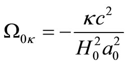
(yet  and curvature is positive). We assumed also that
 , where
  is the parameter of this model and
  is the redshift. We found the optimal values

and
 .
.
The quality of this regression was as high as it was in the  CDM model. Yet the value of
  was much less in the absolute value than in the
  CDM model. The acceleration of the Universe appeared to be a pure observational effect due to the negative pressure.
2. The Equation of Continuity
The Einstein equations with the cosmological constant  are
are
 (1)
(1)
where
• 
• the Einstein gravitational constant [9, p.~347]• 
• the Newton gravitational constant.
To solve these equations we should know the energymomentum tensor . For synchronous coordinates the energy-momentum tensor is
 (2)
(2)
where  is the density of matter and
  is the pressure of matter. The covariant divergence of the energymomentum tensor is zero:
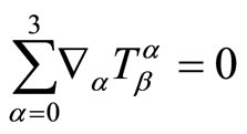 ,
, .
.
If
 ,
, .
.
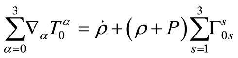
Considering (22) we obtain

for the  component. Assume that the pressure is proportional to the density:
 .
.
for the dust matter this value is  and the value for radiation is
  [9, p.~123]. Therefore

and
 (3)
(3)
Considering physical dimensions of values, the Equation (3) is better as
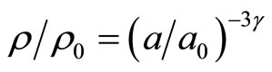 .
.
Hence
 .
.
Let us compare this equation with the change of volume of the Universe for closed models. The FriedmannRobertson-Walker metric in the cosmic time and in the polar coordinates is
 (4)
(4)
where
 ,
,  ,
, 
and  is the curvature parameter
 . The 3-volume element at
  is
is
 .
.
The volume of the Universe at  is
is
 (5)
(5)
Since our Universe is homogeneous, the total amount of matter in the Universe at some  is
is
 (6)
(6)
where . Hence for
  and
and  sufficiently small the total amount of matter in the Universe will be negligible:
  when
when  and
and . Cosmology with
  violates the law of conservation of matter (conservation of leptonic and baryonic numbers [10]). The idea that matter originated from radiation is not a good idea because
  is too large. The matter - antimatter asymmetry also cannot be explained in this way. Cosmology with negative pressure
  contained a “smooth bounce” from the collapsing to expanding stage and this was also due to the same fact. Since the matter disappeared, the gravitation force was negligible and we obtained the smooth bounce with the horizontal tangent [11-13]. The only equation which is fully consistent with (5) and conservation of leptonic and baryonic numbers is
 (7)
(7)
This is due to the equation . The Equation (3) could work for the appropriate epoch only.
Let us try to interpret the covariant divergence of the  4-vector. If currents are negligible (as in the comoving frame), then

will get an additional nonzero component and  will increase or decrease additionally. It seems reasonable because
  is the energy and its change is the redshift. Hence this equation should give a contribution to the redshift (and not bound the matter components). Since

and

due to (5), this covariant divergence is

where  is the pressure. Assume that
 (8)
(8)
Here

is the energy density per unit volume. Integrating

with , we obtain
 (9)
(9)
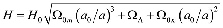
Since the Hubble law is

and both contributions seem to be multiplicative, we get
 (10)
(10)
Hence the redshift depends on the matter equation of state. This correction to redshift  may be useful in cosmology.
3. Correction to the Distance Due to Pressure
3.1. The Hubble Diagram
Recall the distance formula. Define  -coordinate by
 ,
, .
.
Then  if
if  and
and 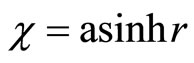 if
if . Hence
  where
where
 (11)
(11)
The Friedmann-Robertson-Walker metric in the cosmic time becomes

The space part of the metric is
 .
.
If  and
and  then
then  and
and . For a photon
 , therefore
 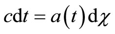 and
and
 (12)
(12)
where
 .
.
Now we use our main hypothesis:
 .
.
Then
 .
.
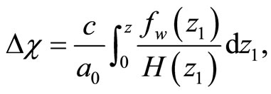
The value of  is the function of
 , therefore

where
 (13)
(13)
Finally
 (14)
(14)
where
 (15)
(15)
Suppose a source has an absolute luminosity , its luminosity (bolorimetric) distance is defined in terms of the measured flux
 (16)
(16)
The measured flux is
 (17)
(17)
one factor of  arising from the decrease in total energy due to the red shift of the energy of the individual photons, and the other factor of
  arising from the increased time interval between the detection of incoming photons due to the fact that two photons separated by a time
  at emission, will be separated by a time
  at the time of detection, where
 [14, p.~41].
hence

and
 .
.
applying our main hypothesis (10) we get
 .
.
recalling the definition of
we get
 for
for .
.
therefore the luminosity distance is
 (18)
(18)
We compared this model with the experimental data of the Supernova Cosmology Project Supernova Ia compilation1. In general no more than two parameters can be determined from these statistical problems [15]. We assumed that  and
and , hence
(yet  and curvature is positive). We assumed also
 (19)
(19)
where  is the parameter of this model. We found the optimal values
and
 .
.
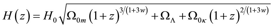
the Hubble diagram with these parameters is presented on the figure 1. The quality of this regression is as high as it is in the ΛCDM model. High values of the mass density are consistent with the experimental data on Supernova Ia within this model. Yet the value of  is much less in the absolute value than in the ΛCDM model.
The Taylor expansion of the luminosity distance (18) is
 (20)
(20)
The optimal values for this simplified case for  are
are

and
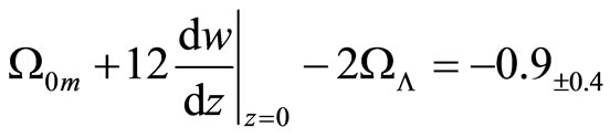 .
.
 (a)
(a)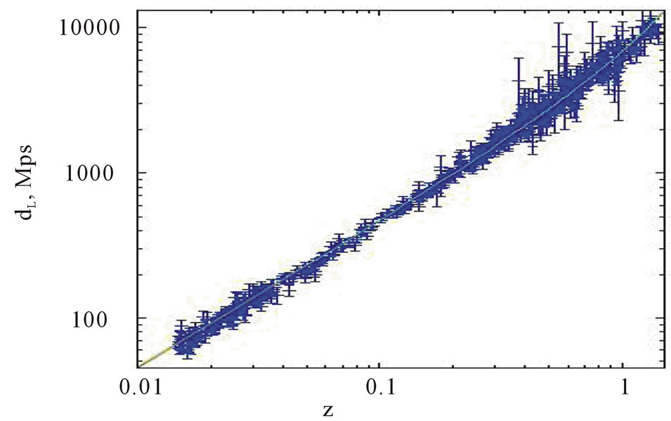 (b)
(b)
Figure 1. The hubble diagram.
3.2. Comparing with the Riess Expansion
In the flat Universe  we can compare (20) with the Equation (10) in [16, p.~25]:
 (21)
(21)
therefore the retardation parameter
 .
.
If the parameter introduced in this paper
 we obtain acceleration. Hence the acceleration of the Universe appears as a pure observational effect due to the negative pressure.
3.3. Fate of the Universe
Note that we have chosen  and
and  while interpreting the Supernova Ia experimental data. We had to make some assumptions on these parameters because large number of unknown parameters cannot be obtained from this simple regression. Yet since experimental data are consistent with
  and
and , then one can say that there is a solution of the Friedman equation wich accelerates for a short time in the beginning but there is a limit for the scale factor
 . We can smoothly glue another solution where the Universe shrinks.
The question of the fate of matter at the end of the Universe is the most complicated. We assume that the matter does not disappeared at the end of the Universe. The matter with some unknown critical density should reproduce the hydrogen and provide condition for another Big Bung. The remnants of the Big Bung are black holes. We assume that all their singularities are topologically equivalent and lead to the same space-time moment in the past where the collapsing stage of the previous Universe ends and the new Big Bung begins.
4. The Section Curvatures
For completeness let us review the Christoffel symbols for the Friedmann-Robertson-Walker metric (4) and the section curvatures. The Christoffel symbols for the timelike dimension (i,j = 1,2,3) are
 (22)
(22)
and ,
, . The Christoffel symbols for the spacelike dimensions are
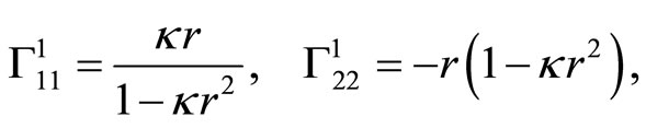


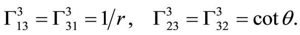
these are all the nonzero components.
Let  be linear independent vectors of the tangent space for the manifold
  at the point
 . The section curvature
  is defined as
 (23)
(23)
where  is the Riemannian curvature map [17, p.~94]. Compared with the Riemannian case we have changed sign in this formula because the signature of our space is Lorentzian. With local coordinates
 .
.
Angle brackets mean scalar product. The denominator is the square of the area of the parallelogram based on the vectors  and
and . If we choose another basis in the same two-dimensional plane
  defined by
  and
and , then the section curvature does not change. Hence the value
  depends on the plane
  only. Therefore the value
  is assigned
  and is called the section curvature of the (pseudo)Riemannian manifold
  at the point
  in the two-dimensional direction
 . In local coordinates the section curvature in the direction
  −
−  is
is
(no summation for ). The section curvature of the FRW space in the directions 0 - 1, 0 - 2, 0 - 3 is
 .
.
In general for any vectors  such as
 ,
,  ,
,  the section curvature
 . The section curvature of the FRW space in the directions 1 - 2, 1 - 3, 2 - 3 is
 .
.
Also for any vectors  such as
  and
and  (other components are arbitrary),
 .
.
Please note that for  and
and  the section curvatures of the spacetime at present are zero. Indeed for the directions 1 - 2, 1 - 3, 2 - 3 the section curvatures
 .
.
It seems sensible that without matter the spacetime should be flat. The section curvatures for the directions 0 - 1, 0 - 2, 0 - 3 are  where
where  is the retardation parameter. At present time
 .
.
In the absence of matter at present for  it will be zero also.
5. Conclusion
We propose new correction to the Hubble's law which can be useful in cosmology. This correction and our assumption  produce a model which is capable to explain the acceleration of our Universe. This model is also consistent with the parameters
  and
and  corresponding to nearly flat and topologically closed Universe. The value
  means that the expansion of the Universe will change to shrinkage yet we should observe acceleration at present. The assimmetry between matter and antimatter is also explained within this model. The matter does not appear from nothing at the beginning of the Universe; it is the same matter that worked at the previous cycle. The matter does not dissappear at the end of the Universe; it will just reproduce the hydrogen. The antimatter is not holes in the Dirac sea of states with negative energy; it is the matter with opposite set of quantum numbers. During the final state of the cycle (which is equally the first state of the new cycle) all properties of matter are equalized.
REFERENCES
- A. A. Friedmann, “Selected Works,” Moscow, Nauka, 1966 (in Russian).
- P. Coles and F. Lucchin, “Cosmology. The Origin and Evolution of Cosmic Structure,” 2nd Edition, John Wiley and Sons, 2002.
- P. J. E. Peebles, “Principles of Physical Cosmology,” Princeton University Press, Princeton, 1993.
- M. Dalarsson and N. Dalarsson, “Tensor Calculus, Relativity and Cosmology,” Elsevier, Amsterdam, 2005.
- S. Weinberg, “Gravitation and Cosmology. Principles and Applications of the General Theory of Relativity,” John Wiley and Sons, Hoboken, 1972.
- B. Ratra and M. S. Vogeley, “Resource Letter: The Beginning and Evolution of the Universe”. arXiv:0706.1565v2.
- R. Kessler, et al., “First-Year Sloan Digital Sky Survey-II (SDSS-II) Supernova Results: Hubble Diagram and Cosmological Parameters”. arXiv:0908.4274v1.
- P. Creminelli, M. A. Luty, A. Nicolis and L. Senatore, “Starting the Universe: Stable Violation of the Null Energy Condition and Non-Standard Cosmologies”. arXiv:hep-th/0606090v2.
- L. D. Landau and E. M. Lifshits, “Course of Theoretical Physics. V. 2. The Classical Theory of Fields,” Moscow, Nauka, 1988 (in Russian).
- L. Wolfenstein, T. G. Trippe and C.-J. Lin, “Tests of Conservation Laws,” The Review of Particle Physics. urlhttp://pdg.lbl.gov.
- Y.-F. Cai, T. Qiu, Y.-S. Piao, M. Li and X. Zhang, “Bouncing Universe with Quintom Matter”. arXiv:0704.1090v1.
- E. A. Bergshoeff, et al., “Cosmological D-Instantons and Cyclic Universes”. arXiv:hep-th/0504011v2.
- D. H. Lyth, “The Primordial Curvature Perturbation in the Ekpyrotic Universe”. {arXiv:hep-ph/0106153v3.
- E. W. Kolb and M. S. Turner, “The Early Universe,” Addison Wesley, Boston, 1990.
- M. Szydlowski, A. Kurek and A. Krawiec, “Top Ten Accelerating Cosmological Models”. arXiv:0604327v2.
- A. G. Riess, et al., “Type Ia Supernova Discoveries at
 from the Hubble Space Telescope: Evidence for Past Deceleration and Constraints on Dark Energy Evolution”. arXiv:0402512v2.
 - Y. D. Burago and V. A. Zalgaller, “Introduction in Riemannian Geometry,” St.-Petersburg, Nauka, 1994 (in Russian).
NOTES
1http://supernova.lbl.gov/Union/figures/SCPUnion2.1_mu_vs_z.txt