 Journal of Environmental Protection, 2011, 2, 873-881 doi:10.4236/jep.2011.27099 Published Online September 2011 (http://www.SciRP.org/journal/jep) Copyright © 2011 SciRes. JEP 873 Henry’s Equilibrium Partitioning between Ground Water and Soil Air: Predictions versus Observations Jeroen Provoost1, Robbe Ottoy2, Lucas Reijnders3, Jan Bronders1, Ilse Van Keer1, Frank Swartjes4, Daniel Wilczek1, David Poelmans1 1Flemish Institute for Technological Research (VITO), Antwerp, Belgium; 2Department PIH, Hogeschool West-Vlaanderen, West Flanders, Belgium; 3Department of Science, Open University Netherlands (OUNL), Netherlands; 4National Institute for Public Health and the Environment (RIVM), Netherlands. Email: Jeroen.Provoost@yahoo.co.uk Received July 3rd, 2011; revised August 5th, 2011; accepted September 6th, 2011. ABSTRACT Humans spend 64% - 94% of their time indoors; therefore, indoor air quality is very important for potential exposure to volatile organ ic compound s (VOC). The source of VOC in the subsurface may come from accidental or intentional re- leases, leaking land fills or leaking und erground and abo ve-ground storage tanks. Once these contaminan ts are present near or beneath buildings, they may move as a vapour through soil gas and enter the building. A large number of va- pour intrusion (VI) algorithms have been published in peer-reviewed publications that link indoor VOC concentrations to the contamination of so ils. These models typically include phase partitio ning calculations of VOC based on Henry’s law to estimate the con centration of a particular con taminant in soil gas. This paper presents the results from a series of laboratory experiments concerning the use of the Henry’s Law constant for the calculation of toluene concentrations in equilibrium between grou nd water and soil air. A series of column experiments were conducted with various toluene concentrations in artificial (ground) water to contrast the predicted and observed (soil) air concentrations. The ex- periments which exclude soil material show a toluene fugacity behaviour roughly in line with Henry’s law whereas the experiments which include soil material result in equilibrium soil concentrations which were around one or- der-of-magnitude lower than was expected from a Henry Law-based estimation. It is concluded that for toluene inclu- sion of Henry’s Law in VI algorithms does not provide an adequate descriptio n of vola tilisa tion in so ils and may lead to an overestimation of health risk. Instead, a model based on a simple description of the relevant intermolecular interac- tions could be explored. Keywords: Henry Law Coefficient, Equilibrium Partitioning, Ground Water, Soil Air, Toluene, Algorithm 1. Introduction During the last two decades, soil and ground water contaminated with volatile organic compounds (VOCs) have received increased attention because of their po- tential to migrate to indoor air and cause human health problems [1-3]. Humans spend on average 80% of their time indoors, ranging from 64% to 94%; therefore, indoor air quality is very important for potential expo- sure to VOCs [4-6]. Swartjes [7] demonstrated that the variation in exposure through indoor air inhalation is comparable to variations in the concentration in indoor air. This suggests that the parameters controlling the variation in the concentration in indoor air, resulting in VOC migration into indoor air (i.e. ‘vapour intrusion’), also control variations in exposure through indoor air inhalation. ‘Vapour intrusion’ (VI) refers to the trans- port of VOC vapours from ground water or soil into buildings. The source of organic vapours in the sub- surface can come from accidental or intentional re- leases [8,9], leaking landfills [10], leaking underground and above-ground storage tanks [11] or related to dry cleaning facilities [12,13]. Once VOCs are introduced into the subsurface, a complex series of fate and trans- port mechanisms act, potentially moving them away from the source area. The distribution of VOCs in soil 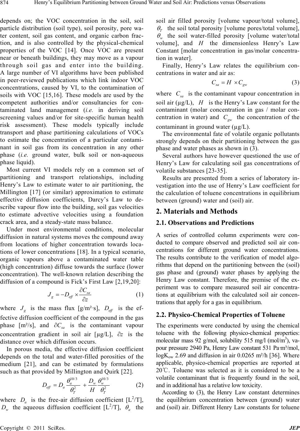 Henry’s Equilibrium Partitioning between Ground Water and Soil Air: Predictions versus Observations 874 depends on; the VOC concentration in the soil, soil particle distribution (soil type), soil porosity, pore wa- ter content, soil gas content, and organic carbon frac- tion, and is also controlled by the physical-chemical properties of the VOC [14]. Once VOC are present near or beneath buildings, they may move as a vapour through soil gas and enter into the building. A large number of VI algorithms have been published in peer-reviewed publications which link indoor VOC concentrations, caused by VI, to the contamination of soils with VOC [15,16]. These models are used by the competent authorities and/or consultancies for con- taminated land management (i.e. in deriving soil screening values and/or for site-specific human health risk assessment). These models typically include transport and phase partitioning calculations of VOCs to estimate the concentration of a particular contami- nant in soil gas from its concentration in any other phase (i.e. ground water, bulk soil or non-aqueous phase liquid). Most current VI models rely on a common set of partitioning and transport relationships, including Henry’s Law to estimate water to air partitioning, the Millington [17] (or similar) approximation to estimate effective diffusion coefficients, Darcy’s Law to de- scribe vapour flow into the building, soil gas velocities to estimate advective velocities using a foundation crack area, and a steady-state mass balance. Under most environmental conditions, molecular diffusion in natural systems moves the compound away from locations of higher concentration towards loca- tions of lower concentrations [18]. In a typical scenario, organic vapours above a contaminated water table (high concentration) diffuse towards the surface (lower concentration). The well-known relation describing the diffusion of a compound is Fick’s First Law [2,19,20]: a geff C JD z (1) where is the mass flux [g/m²·s], is the ef- fective diffusion coefficient of the compound in the gas phase [m²/s], and eff D a C is the contaminant vapour concentration gradient in soil air [µg/L], is the distance over which diffusion occurs. z In porous media, the effective diffusion coefficient depends on the total and water-filled porosities of the medium [21], and can be estimated by formulations such as that provided by Millington and Quirk [22]. 10/3 10/3 2 aw eff a TT D DD H 2 w (2) where a is the free-air diffusion coefficient [L2/T], the aqueous diffusion coefficient [L2/T], D w Da the soil air filled porosity [volume vapour/total volume], T the soil total porosity [volume pores/total volume], w the soil water-filled porosity [volume water/total volume], and the dimensionless Henry’s Law Constant [molar concentration in gas/molar concentra- tion in water]. Finally, Henry’s Law relates the equilibrium con- centrations in water and air as: a CHC gw (3) where a C is the contaminant vapour concentration in soil air (µg/L), is the Henry’s Law constant for the contaminant (molar concentration in gas / molar con- centration in water) and w C the concentration of the contaminant in ground water (µg/L). The environmental fate of volatile organic pollutants strongly depends on their partitioning between the gas phase and water phases as shown in (3). Several authors have however questioned the use of Henry’s Law for calculating soil gas concentrations of volatile substances [23-35]. Results are presented from a series of laboratory in- vestigation into the use of Henry’s Law coefficient for the calcu lation of toluene co ncentra tions in eq uilibriu m between (ground) water and (soil) air. 2. Materials and Methods 2.1. Observations and Predictions A series of controlled column experiments were con- ducted to compare observed and predicted soil air con- centrations for different ground water concentrations. The results contribute to the verification of model algo- rithms that depend on the partitioning between the (soil) gas phase and (ground) water phases by applying the Henry Law constant. Therefore, the premise of the ex- periment was to compare measured soil air concentra- tions at equilibrium with the calculated soil air concen- trations that apply for a gas in equilibriu m. 2.2. Physico-Chemical Properties of Toluene The experiments were conducted by using the chemical toluene with the following physico-chemical properties: molecular mass 92 g/mol, solubility 515 mg/l (mol/m3), va- pour pressure 2940 Pa, Henry Law constan t 531 Pa·m³/mo l , logKow 2.69 and diffusion in air 0.0265 m²/h [36]. Where applicable, physico-chemical properties are reported at 20℃. Toluene was selected as it is considered to be a volatile contaminant that is frequently found in the soil, and in additional has a relative low toxicity. According to (3), the Henry Law constant determines the equilibrium concentration between (ground) water and (soil) air. Different Henry Law constants for toluene Copyright © 2011 SciRes. JEP  Henry’s Equilibrium Partitioning between Ground Water and Soil Air: Predictions versus Observations Copyright © 2011 SciRes. JEP 875 were collected from previously published material at 20℃ [37]. All obtained Henry Law constants were used as input for the calculation of a range of (soil) air concen- trations. Mackay [37] reported 23 different Henry Law constants for toluene that rang from 518 Pa·m³/mol to 825 Pa·m³/mol with a mean of 656 Pa·m³/mol. Henry Law constants were only included in Mackay after the measuring method of the Henry Law constant was veri- fied and appropriate. 2.3. Column Experiments 2.3.1. Setup Figure 1 provides a schematic diagram of the experi- mental set-up. The column was made out of inert glass and the top and bottom plate out of stainless steel. The high-density polyethylene sealing rings prevented leak- age of water or soil air and were non-permeable for VOC. A septum was inserted to allow samples to be taken from the soil air, and air just above the soil surface, without disturbing the equilibrium air concentration in the col- umn. 2.3.2 Procedure For a series of ground water concentrations, duplicate experiments were conducted and all used the same level (volume) of soil and ground water in both columns (Fig- ure 1(a)). The duplicate experiments were used to esti- mate variability as a result of the co lumn setup and sam- pling and to verify that the results are consistent. As the Henry Law constant (3) applies to the equilib- rium partitioning between (ground) water and (soil) air, another series of experiments was conducted without soil material in both columns (Figure 1(b)) to determine the effect of the soil matrix on the vapour equilibrium con- centration. It is assumed that the experiments with and without soil result in similar (soil) air concentrations, as this assumption forms the basis for the implementation of the Henry Law constant in most current VI models. The room temperature where the column experiments were conducted was kept constant at 20℃ (± 1℃) and measured during the full length of the exp eriments. The characteristics of the soil were determined by ap- plying several techniques. The soil bulk density and po- rosity were derived from gravitational measurement of Kopecký’s ring (100 cm3) [38] filled with the soil. This resulted in a soil bulk density of 1758 kg/m³, total poros- ity 0.34, water filled porosity 0.06 and air filled porosity of 0.28. The sieve analysis procedure, or gradation test, is used to assess the particle size distribution, also called gradation, of a granular material, and allows the deter- mination of the soil type. The procedure is described in [39]. Figure 2 reveals that most of the soil particles had a diameter between 300µm and 850 µm which results ac- cording to the soil classification scheme [40] in a very coarse sand. The organic matter content was obtained by first dry- ing 30 gram of soil at 110℃ for 8 hours after which 10 gram of dried soil was put in a container and heated up till 500℃ [41]. The weight before and after glowing represents the organic matter content. This procedure resulted in an organic matter content of 0.21% which was considered to be very low as a natural soil contains Figure 1. Schematic diagram of the experimental column set-up with soil A and without soil B. 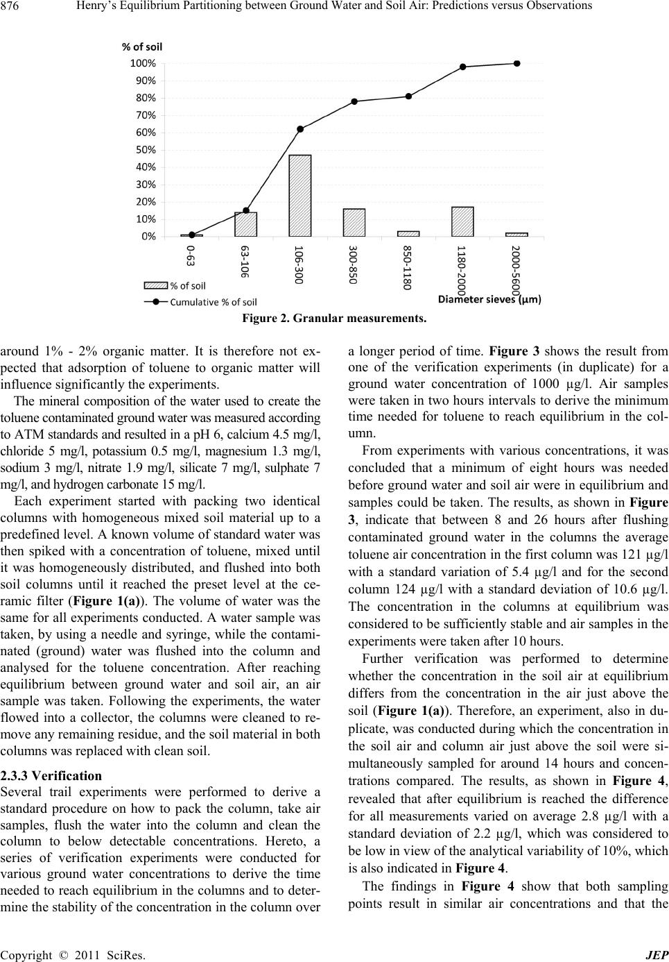 Henry’s Equilibrium Partitioning between Ground Water and Soil Air: Predictions versus Observations 876 Figure 2. Granular measurements. around 1% - 2% organic matter. It is therefore not ex- pected that adsorption of toluene to organic matter will influence significantly the experiments. The mineral composition of the water used to create the toluene contaminated ground water was measured according to ATM standards and resulted in a pH 6, calciu m 4.5 mg/l, chloride 5 mg/l, potassium 0.5 mg/l, magnesium 1.3 mg/l, sodium 3 mg/l, nitrate 1.9 mg/l, silicate 7 mg/l, sulphate 7 mg/l, and hydrogen carbonate 15 mg/l. Each experiment started with packing two identical columns with homogeneous mixed soil material up to a predefined level. A kno wn volume of standard water was then spiked with a concentration of toluene, mixed until it was homogeneously distributed, and flushed into both soil columns until it reached the preset level at the ce- ramic filter (Figure 1(a)). The volume of water was the same for all experiments conducted. A water sample was taken, by using a needle and syringe, while the contami- nated (ground) water was flushed into the column and analysed for the toluene concentration. After reaching equilibrium between ground water and soil air, an air sample was taken. Following the experiments, the water flowed into a collector, the columns were cleaned to re- move any remaining residue, and the so il material in bo th columns was replaced with clean soil. 2.3.3 Verification Several trail experiments were performed to derive a standard procedure on how to pack the column, take air samples, flush the water into the column and clean the column to below detectable concentrations. Hereto, a series of verification experiments were conducted for various ground water concentrations to derive the time needed to reach equilibrium in the columns and to deter- mine the stability of the concentration in the co lumn ov er a longer period of time. Figure 3 shows the result from one of the verification experiments (in duplicate) for a ground water concentration of 1000 µg/l. Air samples were taken in two hours intervals to derive the minimum time needed for toluene to reach equilibrium in the col- umn. From experiments with various concentrations, it was concluded that a minimum of eight hours was needed before ground water and soil air were in equilibrium and samples could be taken. The results, as shown in Figure 3, indicate that between 8 and 26 hours after flushing contaminated ground water in the columns the average toluene air concentration in the first column was 121 µg/l with a standard variation of 5.4 µg/l and for the second column 124 µg/l with a standard deviation of 10.6 µg/l. The concentration in the columns at equilibrium was considered to be sufficien tly stable and air samples in th e experiments were taken after 10 hours. Further verification was performed to determine whether the concentration in the soil air at equilibrium differs from the concentration in the air just above the soil (Figure 1(a)). Therefore, an experiment, also in du- plicate, was conducted during which the concen tration in the soil air and column air just above the soil were si- multaneously sampled for around 14 hours and concen- trations compared. The results, as shown in Figure 4, revealed that after equilibrium is reached the difference for all measurements varied on average 2.8 µg/l with a standard deviation of 2.2 µg/l, which was considered to be low in view of the analytical variability of 10%, which is also indicated in Figure 4. The findings in Figure 4 show that both sampling points result in similar air concentrations and that the Copyright © 2011 SciRes. JEP 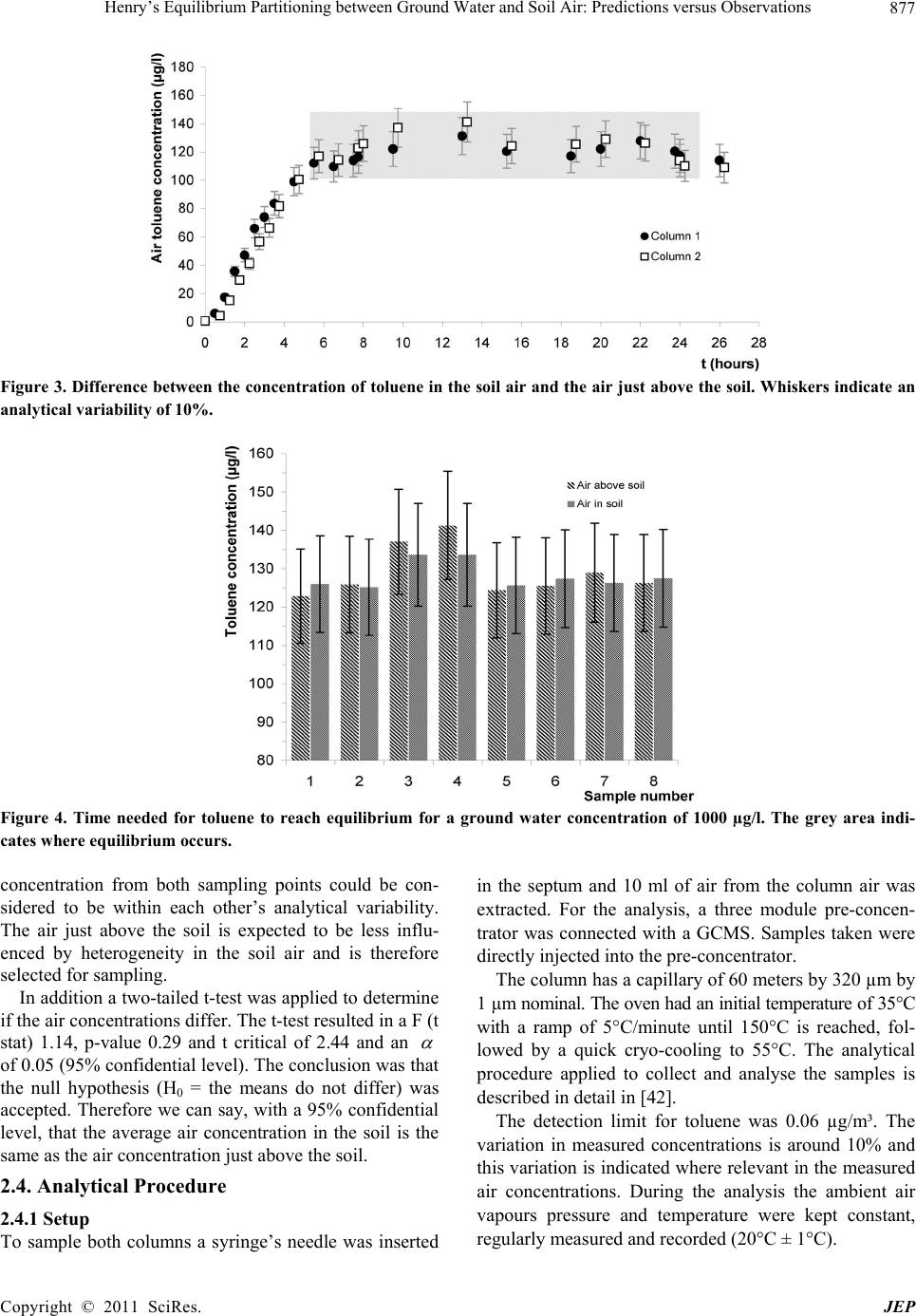 Henry’s Equilibrium Partitioning between Ground Water and Soil Air: Predictions versus Observations 877 Figure 3. Difference between the concentration of toluene in the soil air and the air just above the soil. Whiskers indicate an analytical variability of 10%. Figure 4. Time needed for toluene to reach equilibrium for a ground water concentration of 1000 µg/l. The grey area indi- cates where equilibrium occurs. concentration from both sampling points could be con- sidered to be within each other’s analytical variability. The air just above the soil is expected to be less influ- enced by heterogeneity in the soil air and is therefore selected for sampling. In addition a two-tailed t-test was applied to determine if the air concentrations differ. Th e t-test resulted in a F (t stat) 1.14, p-value 0.29 and t critical of 2.44 and an of 0.05 (95% confidential level). The conclusion was that the null hypothesis (H0 = the means do not differ) was accepted. Therefore we can say, with a 95% confidential level, that the average air concentration in the soil is the same as the air concentration just above the soil. 2.4. Analytical Procedure 2.4.1 Setup To sample both columns a syringe’s needle was inserted in the septum and 10 ml of air from the column air was extracted. For the analysis, a three module pre-concen- trator was connected with a GCMS. Samples taken were directly injected into the pre-concentra tor. The column has a capillary of 60 meters by 320 µm by 1 µm nominal. The oven had an initial temperature of 35°C with a ramp of 5°C/minute until 150°C is reached, fol- lowed by a quick cryo-cooling to 55°C. The analytical procedure applied to collect and analyse the samples is described in detail in [42]. The detection limit for toluene was 0.06 µg/m³. The variation in measured concentrations is around 10% and this variation is indicated where relevant in the measured air concentrations. During the analysis the ambient air vapours pressure and temperature were kept constant, regularly measured and recorded (20°C ± 1°C). Copyright © 2011 SciRes. JEP  Henry’s Equilibrium Partitioning between Ground Water and Soil Air: Predictions versus Observations 878 2.4.2 Calibration Different reference air concentrations for toluene were injected into the GCMS pre-concentrator and further analysed to verify the analytical equipment and to create a calibration line. The calibration line (Figure 5) was then used to derive concentrations of toluene for the in- jected air samples. 2.4. Calculation of the Soil Air Concentration Observed column (soil) air concentrations were com- pared to predicted concentrations. Air concentrations were calculated by using (1) to (3). For each measured ground water concentration a range of predicted air con- centrations were calculated by using the minimum, av- erage and maximum reported Henry Law constant (see Figure 6). 3. Results Figure 6 below displays the data obtained from a series of duplicate experiments for which soil material was in- cluded or excluded from the experiment. For each ex- periment (in the two columns), the toluene ground water concentration was measured in addition to the air con- centrations at equilibrium (10 hours after flushing in the ground water). Comparison of results indicates that a linear increase in air concentration is observed as a result of increasing ground water concentrations. The experiments which exclude soil show a fugacity which is roughly in line with Henry’s Law whereas the experiments which in- clude soil result in around one order-of-magnitude lower air toluene concentration s after reaching equilibriu m than was expected on the b asis of He nry’s law. 4. Discussion This study adds to the argument that partitioning VOCs on the basis of Henry’s Law, as included in current VI algorithms, does not always provide an adequate descrip- tion of experimental data. This is in line with findings from [34] and [43]. A main contribution to divergence form Henry’s law might come from a rate-limiting mass transfer from ground water to soil gas [44,45]. As the present study only regards toluene, additional research into the partitioning of other VOCs is needed to test the more general adequacy of current VI algorithms for vola- tile organic compounds. Equally important is the as- sumption that the soil and groundwater properties were considered to be constant. Under slightly different condi- tions, for example different volumes of soil and ground- water, the results may have varied. For toluene the present study indicates that current use of Henry’s law in VI algorithms may lead to an overes- timation of toluene concentrations in soil gas, which in turn might give rise to an overestimate of potential health Figure 5. Calibration line deriving the peak surface area for various known toluene concentrations. Copyright © 2011 SciRes. JEP  Henry’s Equilibrium Partitioning between Ground Water and Soil Air: Predictions versus Observations879 Figure 6. Observed and pre dicted conce ntrations in the column air for different ground w ater concentrations measured after 10 hours. Data is provided for air concentrations with and without soil material present in the columns. The dotted line indi- cates the average (mean) predicted air concentrations based on the Henry Law constants with the grey area representing the variation. Whiskers indicate the 10% variation in the measured air concentration. risk of toluene intrusion into buildings. While this might be acceptable for screening level assessments, which should be conservative [16,44-46], this is not acceptable for estimates of real life risks. The latter should rather be estimated on the basis of direct measurements of toluene concentrations in indoor air and actual soil, water and soil gaseous phase contamination. The findings presented also indicate the need to improve current VI algorithms. Such improvement might be based on a simple descrip- tion of the relevant intermolecular interactions could as described by [34]. 5. Conclusions This paper shows that column experiments which ex- clude soil show a toluene fugacity behaviour roughly in line with Henry’s law whereas column experiments which include soil material result in around one or- der-of-magnitude lower air concentrations after reaching equilibrium than was expected on the basis of Henry’s law. It is concluded that for toluene inclusion of Henry’s Law in VI algorithms does not provide an adequate de- scription of experimental data and may lead to an overes- timation of health risk. Instead, a model based on a sim- ple description of the relevant intermolecular interactions could be explored. REFERENCES [1] J. Kliest, T. Fast, J. S. M. Boley, H. van de Wiel and H. Bloemen, “The Relationship between Soil Contaminated with Volatile Organic Compounds and Indoor Air Pollu- tion,” Environment International, Vol. 15, No. 1-6, 1989, pp. 419-425. [2] J. C. Little, J. M. Daisey and W. W. Nazaroff, “Transport of Subsurface Contaminants into Buildings. An Exposure Pathway for Volatile Organics,” Environmental Scientific Technology, Vol. 26, No. 11, 1992, pp. 2058-2066. doi:10.1021/es00035a001 [3] F. D. Tillman and J. W. Weaver, “Temporal Moisture Content Variability Beneath and External to a Building and the Potential Effects on Vapour Intrusion Risk As- sessment,” Science of the Total Environment, Vol. 379, 2007, pp. 1-15. [4] M. B. Kaplan, P. Brandt-Rauf, J. W. Axley, T. T. Shen and G. H. Sewell, “Residential Releases of Number 2 Fuel Oil: A Contributor to Indoor Air Pollution,” Ameri- can Journal of Public Health, Vol. 83, No.1, 1993, pp. 84-88. [5] D. Fugler and M. Adomait, “Indoor Infiltration of Vola- tile Organic Contaminants: Measured Soil Gas Entry Rates and Other Research Results from Canadian Copyright © 2011 SciRes. JEP  Henry’s Equilibrium Partitioning between Ground Water and Soil Air: Predictions versus Observations 880 Houses,” Journal of Soil Contamination, Vol. 6, No. 1, 1997, pp. 9-13. doi:10.1080/15320389709383542 [6] D. A. Olson and R. L. Corsi, “Fate and Transport of Con- taminants in Indoor Air,” Journal of Soil and Sediment Contamination, Vol. 11, No. 4, 2002, pp. 583-601. [7] F. A. Swartjes, “Evaluation of the Variation in Calculated Human Exposure to Soil Contaminants Using Seven Dif- ferent European Models,” Human and Ecological Risk Assessment, Vol. 15, No. 1, 2009, pp. 138-158. doi:10.1080/10807030802615733 [8] M. C. Underwood, “Assessing the Indoor Air Impact from a Hazardous Waste Si te: A Case Study,” Toxicology and Industrial Health, Vol. 12, No. 2, 1996, pp. 179-188. [9] B. Eklund, D. Folkes, J. Kabel and R. Farnum, “An Over- view of State Approaches to Vapor Intrusion,” Environ- mental Manager, Air & Waste Management Association, February 2007, pp. 10-13. [10] J. F. Foster and B. D. Beck, “Basement Gas: Issues Re- lated to the Migration of Potentially Toxic Chemicals into House Basements from Distant Sources,” Advanced Mod- elling Environmental Toxicology, Vol. 25, 1998, pp. 219-234. [11] S. Chowdhury and S. L. Brock, “Indoor Air Inhalation Risk Assessment for Volatiles Emanating from Light Nonaqueous Phase Liquids,” Soil and Sediment Con- tamination, Vol. 10, No. 4, 2001, pp. 387-403. [12] M. J. Moran, J. S. Zogorski and P. J. Squllace, “Chlorin- ated Solvents in Groundwater of the United States,” E nvi- ronmental Science and Technology, Vol. 41, No. 1, 2007, pp. 74-81. doi:10.1021/es061553y [13] J. Roy and G. Bickerton, “Proactive Screening Approach for Detecting Groundwater Contaminants along Urban Streams at the Reach-Scale,” Environmental Science and Technology, Vol. 44, No. 16, 2010, pp. 6088-6094. [14] D. R. Williams, J. C. Paslawski and G. M. Richardson, “Development of a Screening Relationship to Describe Migration of Contaminant Vapours into Buildings,” Jour- nal of Soil Contamination, Vol. 5, No. 2, 1996, pp. 141-156. doi:10.1080/15320389609383519 [15] T. McAlary, J. Provoost and H. Dawson, “Chapter 10—Vapour Intrusion,” In: F. Swartjes, Ed., Dealing with Contaminated Sites—From Theory towards Practical Application, Springer Publishers, Netherlands, January 2011, pp. 409-453. [16] J. Provoost, F. Tillman, J. Weaver, L. Reijnders, J. Bronders, I. Van Keer and F. Swartjes, “Chapter 2 Va- pour Intrusion into Buildings—A Literature Review,” In: J. A. Daniels, Ed., Advances in Environmental Research, Nova Science Publishers Inc., New York, 2010, pp. 69-111. [17] R. J. Millington, “Gas Diffusion in Porous Media,” Sci- ence, Vol. 130, No. 3367, 1959, pp. 100-102. doi:10.1126/science.130.3367.100-a [18] H. L. Penman, “Gas and Vapour Movements in Soil I, the Diffusion of Vapours through Porous Solids,” Journal of Agricultural Science, Vol. 30, 1940, pp. 463-462. [19] W. W. Nazaroff, “Radon Transport from Soil to Air, Re- view of Geophysics,” American Geophysical Union, Vol. 30, No. 2, 1992, pp. 137-160. [20] W. A. Jury, W. F. Spencer and W. J. Farmer, “Behavior Assessment Model for Trace Organics in Soil: I. Model Description,” Journal of Environmental Quality, Vol. 12, No. 4, 1983, pp. 558-563. doi:10.2134/jeq1983.00472425001200040025x [21] J. A. Currie, “Movement of Gases in Soil Respiration, Sorption and Transport Processes in Soils,” SCI Mono- graph Series, Vol. 37, 1970, pp. 152-171. [22] R. J. Millington and J. P. Quirk, “Permeability of Porous Solids,” Transactions of the Faraday Society, Vol. 57, 1961, pp. 1200-1207. doi:10.1039/tf9615701200 [23] W. Malesinski, “Azeotropy and Other Theoretical Prob- lems of Vapour-Liquid Equilibrium,” InterScience, 1965, pp. 222. [24] W. F. Spencer, M. M. Cliath, W. A. Jury and L. Z. Zhang, “Volatilization of Organic Chemicals from Soil as Re- lated to their Henry’s Law Constants,” Journal Environ- mental Quality, Vol. 17, No. 3, 1988, pp. 504-509. doi:10.2134/jeq1988.00472425001700030027x [25] J. E. Dunn and T. Chen, “Critical Evaluation of the Dif- fusion Hypothesis in the Theory of Porous Media Volatile Organic Compound (VOC) Sources and Sinks,” In: N. L. Nagda, Ed., Modelling of Indoor Air Quality and Expo- sure, American Society for Testing and Materials, Phila- delphia, 1993, pp. 64-80. [26] A. L. Robinson, R. G. Sexto and W. J. Fisk, “Soil-Gas Entry into an Experimental Basement Driven by Atmos- pheric Pressure Fluctuations—Measurements, Spectral Analysis, and Model Comparison,” Atmospheric Envi- ronment, Vol. 31, No. 10, 1997, pp. 1477-1485. doi:10.1016/S1352-2310(96)00304-4 [27] A. L. Robinson, R. G. Sexto and W. J. Riley, “Soil-Gas Entry into an Experimental Basement Driven by Atmos- pheric Pressure Fluctuations—The Influence of Soil Properties,” Atmospheric Environment, Vol. 31, No. 10, 1997, pp. 1487-1495. doi:10.1016/S1352-2310(97)83264-5 [28] J. Grifoll and Y. Cohen, “Chemical Volatilization from the Soil Matrix—Transport through the Air and Water Phases,” Journal of Hazardous Materials, Vol. 37, No. 3, 1994, pp. 445-457. doi:10.1016/0304-3894(93)E0100-G [29] R. L. Scott, “Azeotropy and Other Theoretical Problems of Vapour-Liquid Equilibrium,” Journal of American Chemistry Society, Vol. 88, No. 21, 1966, pp. 5053. doi:10.1021/ja00973a070 [30] K. U. Goss, “Adsorption of Organic Vapours on Polar Mineral Surfaces and on a Bulk Water Surface: Devel- opment of an Empirical Predictive Model,” Environ- mental Science and Technology, Vol. 28, No. 4, 1994, pp. 640-645. doi:10.1021/es00053a017 [31] K. U. Goss, “Effects of Temperature and Relative Hu- midity on the Sorption of Vapours on Quartz Sand,” En- vironmental Science and Technology, Vol. 26, No. 11, 1992, pp. 2287-2294. doi:10.1021/es00035a030 [32] K. U. Goss and S. J. Eisenreich, “Adsorption of VOCs Copyright © 2011 SciRes. JEP  Henry’s Equilibrium Partitioning between Ground Water and Soil Air: Predictions versus Observations Copyright © 2011 SciRes. JEP 881 from the Gas Phase to Different Minerals and a Mineral Mixture,” Environmental Science and Technology, Vol. 30, No. 7, 1996, pp. 2135-2142. doi:10.1021/es950508f [33] K. U. Goss, J. Buschmann and R. P. Schwarzenbach, “Linear Free Energy Relationships Used to Evaluate Equilibrium Partitioning of Organic Compounds,” Envi- ronmental Science and Technology, Vol. 35, No. 1, 2001, pp. 1-9. doi:10.1021/es000996d [34] K. U. Goss, “The Air/Surface Adsorption Equilibrium of Organic Compounds under Ambient Conditions, Critical Reviews,” Environmental Science and Technology, Vol. 34, No. 4, 2004, pp. 339-389. doi:10.1080/10643380490443263 [35] K. U. Goss, J. Buschmann and R. P. Schwarzenbach, “Adsorption of Organic Vapours to Air-Dry Soils: Model Predictions and Experimental Validation,” Environmental Science and Technology, Vol. 38, 2004, pp. 3667-3673. doi:10.1021/es035388n [36] J. Provoost, J. Nouwen, C. Cornelis, G. Van Gestel and R. Engels, Technical Guidance Document, Part 4—Back- ground Document for Chemical Properties and Specifica- tions, Advise on Behalf of the Flemish Public Waste Agency OVAM, Dutch, 2004. [37] D. Mackay, W.-Y. Shiu, K. C. Ma and S. C. Lee, “Hand- book of Physical-Chemical Properties and Environmental Fate for Organic Chemicals,” Second Edition, Vol. 1-4, CRC Press, 2006. [38] S. Matula, M. Mojrova and K. Spongrova, “Estimation of the Soil Water Retention Curve (SWRC) Using Pe- dotransfer Functions (PTFs),” Soil and Water Research, Vol. 2, No. 4, 2007, pp. 113-122. [39] ASTM, “Astm Standard C136-06 Standard Test Method for Sieve Analysis of Fine and Coarse Aggregates,” ASTM International, West Conshohocken, PA, 2006. doi:10.1520/C0136-06 [40] R. B. Brown, “Soil Texture,” Fact Sheet SL-29, Institute of Food and Agricultural Sciences, University of Florida, 2003. [41] ASTM, “ASTM Standard D2974-07a Standard Test Methods for Moisture, Ash, and Organic Matter of Peat and Other Organic Soils,” ASTM International, West Conshohocken, PA, 2007. doi:10.1520/C0136-06 [42] US EPA, Compendium of Methods for the Determination of Toxic Organic Compounds in Ambient Air, Second Edition, Compendium Method TO-15, Determination of Volatile Organic Compounds (VOCs) in Air Collected in Specially-Prepared Canisters and Analyzed by Gas Chromatography/Mass Spectrometry (GC/MS), Center for Environmental Research Information, Office of Re- search and Development, U.S. Environmental Protection Agency, Cincinnati, 1999. http://www.epa.gov/ttnamti1/airtox.html [43] S. W. Webb and K. Pruess, “The Use of Fick’s Law for Modeling Trace Gas Diffusion in Porous Media,” Trans- port in Porous Media, Vol. 51, 2003, pp. 327-341. [44] J. Provoost, L. Reijnders, F. Swartjes, J. Bronders, P. Seuntjens and J. Lijzen, J, “Functionality and Accuracy of Seven Vapour Intrusion Screening Models for VOC in Groundwater,” Journal of Soil s and Sedi ment s—Protection, Risk Assessment, and Remediation, Vol. 9, 2008. doi:10.1007/s11368-008-0036-y [45] J. Provoost, A. Bosman, L. Reijnders, J. Bronders, K. Touchant and F. Swartjes, “Vapour Intrusion from the Vadose Zone—Seven Algorithms Compared,” Journal of Soils and Sediments—Protection, Risk Assessment, and Remediation, 2009. doi:10.1007/s11368-009-0127-4 [46] P. C. Johnson, M. W. Kemblowski and R. L. Johnson, “Assessing the Significance of Subsurface Contaminant Vapour Migration to Enclosed Spaces: Site-Specific Al- ternatives to Generic Estimates,” Journal of Soil Con- tamination, Vol. 8, 1999, pp. 389-421.
|