Paper Menu >>
Journal Menu >>
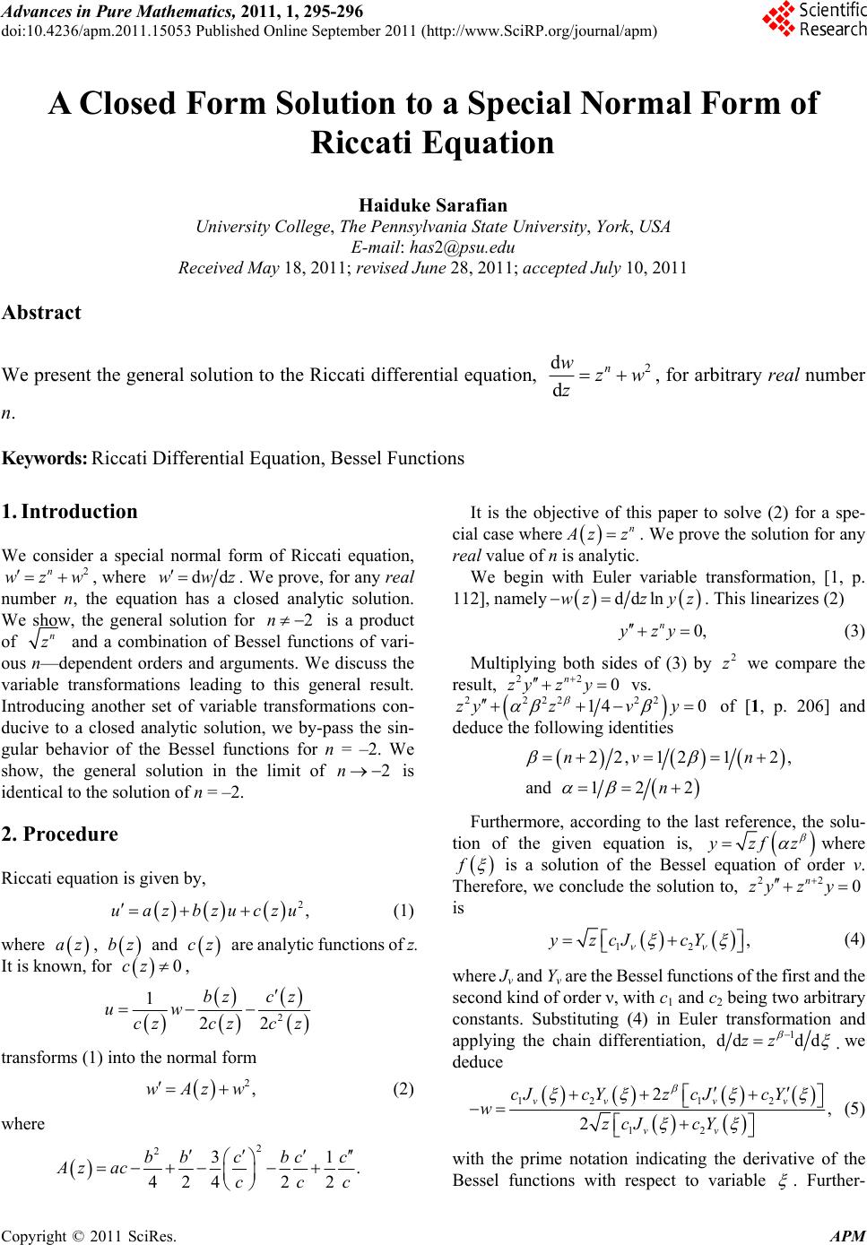 Advances in Pure Mathematics, 2011, 1, 295-296 doi:10.4236/apm.2011.15053 Published Online September 2011 (http://www.SciRP.org/journal/apm) Copyright © 2011 SciRes. APM A Closed Form Solution to a Special Normal Form of Riccati Equation Haiduke Sarafian University College, The Pennsylvania State University, York, USA E-mail: has2@psu.edu Received May 18, 2011; revised June 28, 2011; accepted July 10, 2011 Abstract We present the general solution to the Riccati differential equation, 2 d d n wzw z , for arbitrary real number n. Keywords: Riccati Differential Equation, Bessel Functions 1. Introduction We consider a special normal form of Riccati equation, , where 2n wzw ddww z. We prove, for any real number n, the equation has a closed analytic solution. We show, the general solution for is a product of 2n n z and a combination of Bessel functions of vari- ous n—dependent orders and arguments. We discuss the variable transformations leading to this general result. Introducing another set of variable transformations con- ducive to a closed analytic solution, we by-pass the sin- gular behavior of the Bessel functions for n = –2. We show, the general solution in the limit of is identical to the solution of n = –2. 2n 2. Procedure Riccati equation is given by, 2,uaz bzuczu (1) where , and are analytic functions of z. It is known, for , az bz cz cz 0 2 1 22 bzc z uw czcz cz transforms (1) into the normal form 2,wAz w (2) where 2 231 . 4242 2 bbcbc c Az accc It is the objective of this paper to solve (2) for a spe- cial case where n A zz . We prove the solution for any real value of n is analytic. We begin with Euler variable transformation, [1, p. 112], namely dd lnwzz yz . This linearizes (2) 0, n yzy (3) Multiplying both sides of (3) by we compare the result, 2 z 22 0 n zyz y vs. 2222 22 14 0zyzv y of [1, p. 206] and deduce the following identities 22, 1212, and 122 nv n n Furthermore, according to the last reference, the solu- tion of the given equation is, yzfz where f is a solution of the Bessel equation of order v. Therefore, we conclude the solution to, 22 0 n zyz y is 12 ,yzcJ cY (4) where Jv and Yv are the Bessel functions of the first and the second kind of order ν, with c1 and c2 being two arbitrary constants. Substituting (4) in Euler transformation and applying the chain differentiation, 1 dd ddzz we deduce 12 12 12 2, 2 vv vv vv cJcYz cJcY wzcJ cY (5) c with the prime notation indicating the derivative of the Bessel functions with respect to variable . Further-  H. SARAFIAN 296 more, applying two sets of recurrence relationships [2, p. 361], 11 11 1 2 ,, 2 vv vvv JJ YY JJJJ YYYY v v simplifies (5) 22 22 11 21 22 2 2 11 21 22 22 2, 22 22 nn nn nnn n nn cJzcYz nn wz cJz cYz nn 2 2 2 n (6) And, (6) simplifies to its final form 22 2 11 22 2 22 11 22 22 22 , 22 22 nn nn nn n n nn CJz Yz nn wz CJz Yz nn 2 2n (7) With 12 .Ccc We observe that solution (2) is a one-parameter family function. The n = –2 is the pole of the order and the argument of the Bessel functions and needs a special consideration. For n = –2 Equation (2) takes the form 2 2 1,w z w (8) By inspection, 2 1 w z solves (8). Substituting w in (8) gives . We select 1 210 12 13i to further the analysis. The standard variable transforma- tion [1, p. 50] 1 1 ww z , (9) gives the general solution. Substituting (9) in (8) yields, 1 '21 0,vv z (10) The solution of (10) is, 1 2 1 21cz z , with C being a constant. The solution to (8) yields, 3 11 1 13 1 2 3 i wi zCz i Figure 1. The s olid curve is the graph of the solution given in (12) for c1 = 1. The gray curve is the graph of the solution given in (7) for n = –1.99 and C = 0.85. Applying the identities, ln z zeand 1 tan iz iz iz iz ee zie e and suitably selecting the value of 1 3 3 ci i Ce , (11) becomes 1 13 13cot ln 22 wz z,c (12) We show graphically, see Figure 1, that (7) in the limit of is identical to (12). 2n 3. A comment and an Acknowledgement By applying multiple step variable transformations (not reported in this paper) the author devised a method of solving (2) resulting in (7). The author appreciates the in depth discussion with Prof. Rostamian. 4. References [1] W. E. Boyce and R. C. DiPrima, “Elementary Differential Equations and Boundary Value Problems,” 6th Edition, Wiley, New York, 1997. [2] M. Abramowitz and I. A. Stegun, “Handbook of Mathe- matical Functions,” Dover Publications Inc., New York, 1970. , (11) Copyright © 2011 SciRes. APM |