Modern Economy, 2011, 2, 642-653
doi:10.4236/me.2011.24072 Published Online September 2011 (http://www.SciRP.org/journal/me)
Supply Quantitative Model à la Leontief*
Ezra Davar
Independent Researcher, Amnon Vtamar, Netanya, Israel
Received May 13, 2011; revised July 6, 2011; accepted July 16, 2011
Abstract
This paper focuses on the supply quantitative model system of input–output, which is equivalent to the de-
mand quantitative model system of Leontief. This model allows us to define the total supplied quantities of
commodities for any given supplied quantity of primary factors, and consequently enables us to define the
final uses of commodities. The supply quantitative model is based on the direct output coefficients of pri-
mary factors. The Hadamard Product is also used. The quantitative supply system models might be useful
tools in planning the economics of countries that have higher unemployment of primary factors, especially
labour.
Keywords: Leontief, Demand and Supply Quantitative Model, Output Coefficients, the Hadamard Product
1. Introduction
Leontief used the term “Input-Output” in the title of his
first and seminal paper on Input-Output Analysis, in
“Quantitative Input and Output Relations in the Eco-
nomic System of the United States” [1]. This means that
every activity in economics is simultaneously character-
ized by two sides: income (revenue) expenditure, de-
mand supply, input-output, export-import, and so on. In
other words, the income of a certain economic unit
(household, firm, institution, country) is co ncurrently ex-
penditure for another economic unit; demand for any
commodity by any individual is also supply for another
individual or firm; input of any commodity to a certain
sector is also output for the sector producing that com-
modity. Using this postulate, Leontief describes his in-
put-output table as: ‘Each row contains the revenue (out-
put) items of one separate business (or household) … If
read vertically, column by column, the table shows the
expenditure sides of the successive accounts’ [1]. There-
fore, this allows us to describe and analyze economies on
two sides so that if the same conditions exist, the results
must be equivalent for both—in quantity an d pr ice terms.
For example, the development of the whole economy
might be modeled on either the input side or the output
side. Each direction has its own targets and allows us to
solve different types of problems of contemporary eco-
nomics.
Since that period in economic literature on Input-
Output, there have been attempts to formulate models
describing the whole economy in both sides: demand
(input) and supp ly (ou tput) for quantity and supp ly (input)
and demand (output) for price. Until today, only two
types of system models of input-output have been for-
mulated. These system models were first formulated by
Leontief in their original form, and in the following years
they were improved upon: quantitative demand (input)
and price supply (input) models ([1-4]). The first model
allows us to define the demand (required ) quantity of the
total production (input) of commodities for any given
amount of final uses and consequently also for defining
the demand (required) quantity of the primary factors.
The second model allows us to def ine the cost of produ c-
tion (supply price) of commodities on the basis of pri-
mary factors’ prices which are determined according to
their required quantities by means of their total supply
curves ([5,6]).
When Ghosh ([7,8]) formulated the allocation model,
it was unfortunately labeled into an “output” (supply,
supply-driven) model by his followers ([9-12])1. More-
over, Dietzenbacher ([10]; see also [13]) attempted to
prove that Ghosh’s allocation model is equivalent to Le-
ontief’s price model. However, the recent paper [6]
1I also, unfortunately, finally called Ghosh’s model an output model,
despite the fact that in my first paper [19] the distribution and outpu
t
coefficients (are) were used equivalently, but in my book [5] I men-
tioned ‘distribution coefficients’ only once and after that ‘output coeffi-
cients’ and ‘output models’ were used.
*The author thanks Prof. A. Brody and Prof. E. Einy for useful sugges-
tions; This paper is dedicated to Leontief’s 100th birthday, and 70 years
since his first paper on Input-Output.

E. DAVAR643
shows that Leontief’s Input-Output system model differs
from Ghosh’s system, and therefore they cannot be equi-
valent.
This paper focuses on the supply quantitative model
that allows us to define the total supplied quantities of
commodities for any given supplied quantity of primary
factors, and consequently to define the final uses of com-
modities for both physical and monetary input-output
systems. The supply quantitative model à la Leontief is
based on the output coefficients of primary factors and
input coefficients of commodities. The output coeffi-
cients of primary factors are the inverse magnitudes of
their inputs coefficients; therefore, if the input coeffi-
cients are given and constant by assumptions, then the
output coefficients are also given and constant. The Ha-
damard Product is also used.
Hence, this model allows us to define the total sup-
plied quantities of commodities for any given supplied
quantity of primary factors, and consequently to define
the final uses of commodities. Such approach allows us
to manipulate by each components of primary factor
(types of labour or fixed capital). While Ghosh’s model
is based on the allocation coefficients of commodities,
which are not inverted of the input coefficients, and on
the input coefficients of primary factors, and therefore,
allows manipulate generally by an aggregate magnitude
of value added.
This paper consists of two sections. Following the in-
troduction the first section describes supply quantitative
equilibrium system models for Input-Output in physical
terms; and the second section deals with supply quantita-
tive equilibrium system models for Input-Output in mo-
netary terms. Finally conclusions are presented.
2. Supply Quantitative Equilibrium for I-O
in Physical Terms à la Leont ief2
Let us start with the demand quantitativ e model of Leon-
tief’s input-output system, before describing the supply
quantitative mod el, for two reasons: (1) to consider addi-
tional property of the demand model; and (2) to compare
and understand characteristics of these models. The de-
mand quantitative equilibrium for I-O in physical terms
consists of two systems [6]:


1
,or ,or
dddddd d
x
AxyxIAyxBy

 (1.1)

0
0
ˆ
or
ddd
nn
dd d
vVi CxiCxv
vCxCByv
 
  (1.2)
where
ij
X
x




—is the square matrix (n*n) of the quantita-
tive flows of commodities in the production;
ir
Yy




—is the matrix (n*R) of the quantitative
flows of commodities to the categories of final uses;
d
y– is the column vector (n*1) of commodities’
quantities for final uses;
d
x
—is the column vector (n*1) of the total output
quantity of commodities;
kj
Vv




—is the matrix (m*n) of the quantitative
flows of primary factors to the sectors of production;
d
v– is the column vector (m*1) of the total quantities
of primary factors required in the production ;
ij
A
a




—is the square matrix (n*n) of the direct in-
put coefficients of commodities in real (physical) terms
in the production and

1
ˆ,.., ij
dij d
j
x
AXx iea
x

; (1.3)
i.e., the input coefficient aij measure quantity of com-
modity i required for the production of one unit of com-
modity j in physical terms;
kj
Cc




—is the matrix (m*n) of the direct input co-
efficients of factors in real physical terms in the produc-
tion and

1
ˆ,.., kj
dkj d
j
v
CVx iec
x

; (1.4)
i.e., the input coefficient of primary factors kj c
measure quantity of factor k required for the production
of one unit of commodity j in physical terms;
B—is Leontief’s inverse matrix, and ij bis the total
required quantities (direct and indirect inputs) of com-
modity i to a satisfied one unit of demand of the com-
modity j;
—
0
v—is the vector of the available quantities of pri-
mary factors;
n
The system (1.1) allows us to obtain the total requ ired
quantities of commodities for any given quantities of
final uses for the certain conditions of the direct input
coefficients of commodities
i—is a unit column vector (n*1);
A
. Consequently, by the
substitution of the obtained required output quantities in
the system (1.2), the required quantities of primary fac-
tors are defined as d v. Therefore, if the required quanti-
ties of primary factors are within the limit quantities
drawing from their supply curves, i.e., if the required
quantities are less or equal to the available quantities
(0
d
vv

), then there is a quantitative equilibrium and
then a price equilibrium establishing might be considered.
2Input-Output in physical terms, in this paper, differs from the physical
input-output table (PIOT), which recently appeared in input-output
literature. In the former, each commodity has its own physical meas-
urement: meter, ton, unit, M3 and so on, while in the latter, all com-
modities have uniform physical measu
r
ement, for example ton.

E. DAVAR 644
Conversely, when, if at least the required quantity for
one factor is larger than its available quantity, then the
process must be carried out for the new different quanti-
ties for final uses, until the above conditions are satisfied.
Worthy to discuss the character of changes of the total
required quantities of primary factors due to change of
quantities of final uses. We assume, for the simplifica-
tion, that only th e quantity o f final us e for a on e of sector
(commodity) l is changed (increased) (d
l), while the
final uses for other sectors (commodities) stay un-
changed. Substitute this in (1.1), and we have:
y

11dd dddd
x
ByB yyxx  (1.5)
where d
y—is the column vector (n*1) all components
of which are zer o exce pt of the compo nent l that equ al to
d
l
y. So
dd
x
By (1.6)
and

,,1,2,
dd
iij
l
x
byjli n  (1.7)
From (1.7) we can conclude that increasing the final
use of the commodity of a certain sector l either in-
creases the total production of commodities of the se-
ctors where according inverse coefficients of inputs are
more than zero (bij > 0, j = l) or unchanged if according
inverse coefficients of inputs equal zero (bij = 0, j = l).
Consequently, the qu antities of primary factors are either
increased, if direct input coefficients of primary factors
are more than zero (ckj > 0), or unchanged if direct input
coefficients of primary factors are equal to zero (ckj = 0)
in the sectors where the total production is increased.
This is


,1,2,,;1,2,,
d
kjkjji ll
vcb ykmjn

 

(1.8)
Now, the total increase of each primary factor is de-
termined as


11 ,1,2,,
dd
nn
jj
kkjkjjil
l
vvcbyk
 
 

m (1.9)
From (1.9) d
l
yis determined as

1
dd
n
j
kkjj
l
yv cb

il (1.10)
However, these total increases of each primary factor
must be less or equal to its unemployed quantities, this
is:


0,1,2,,
dd
kk k
vvvk m  (1.11)
Therefore


0
11
max minn
dd
kk kjji
lkm j
yvvcb

 
 l , (1.12)
This proves the following theorem:
Theorem 1 If matrix A is positive (A  0) and produc-
tive (x > xA), and if the quantity of final use of a certain
sector d yl is increased and final uses for all other sec-
tors are unchanged, then the required quantities of pri-
mary factors are either increased if direct input coeffi-
cients of primary factors are more than zero (ckj > 0) or
unchanged if direct input coefficients of primary factors
are equal to zero (ckj = 0) for the sectors where the total
production is increased; also the magnitude of the in-
crease of final use of a certain sector (commodity) is
limited by the unemployed supply quantities of primary
factors (1.12).
To sum up, this theorem indicates that increasing of
the quantity in the final use of the commodity of a certain
sector, increases the required quantities of primary fac-
tors almost in all sectors.
On the other hand, careful examination of the demand
system models shows that they might be used for oppo-
site purposes (direction) too. Namely, the system (1.1)
might be used to obtain the total quantities of final uses
for any given total quantity of commodities, rewriting it
as:

d
yIAx d (1.13)
So, (1.13) allows us to obtain the total quantity of final
uses for a given total quantities of commodities. This
means that in order to determine the total demand of fi-
nal uses, the total quantities of commodities have to be
known, so that the latter have to be connected with pri-
mary factors. For example, the total quantities of com-
modities must be determined on the basis of the given
quantities of primary factors. In other words, the oppo-
site model to (1.2) is required.
The question is, therefore, whether the system (1.2)
may be transformed into such a model which may allow
us to determine the total quantities of commodities for
any given quantities of primary factors. Until today, the
answer was obviously negative. It asserted that the co-
lumn of primary factors for a certain sector, for the input-
output system in physical terms, is heterogeneous and
therefore, not be summed. Thus the negative answer is
based on the ordinary analysis of input-output system
models.
Let us try another approach.
Let’s start from the determination of the flows of pri-
mary factors to sectors of production (V—matrix). From
(1.2) it is determined that:
ˆ
d
VCxd (1.14)
If we take into account the fact that when regular ma-
trix is multiplied on a diagonal matrix, it means that the
first component of each row of regular matrix is multi-
plied on the element of the first column of the diagonal

E. DAVAR645
matrix and the second element of each row is multiplied
on the element of the second column, and so on. There-
fore, the diagonal matrix may be replaced by a matrix
where all elements of a certain column are identical and
equal to the according diagonal magnitude; and new ma-
trix’s dimension is defined according to the dimension of
matrix C, i.e. (m*n). This is, taking case ˆd
x
under dis-
cussion, might be replaced by the matrix dd
X
(m*n)
where all elements of the first column would be the total
output of the first sector, all elements of the second co-
lumn – the total output of the second sector, and so on:
11 121
21 222
12
dd dn
dd dn
dd
dm dmdmn
xx x
xxx
X
xx x


















(1.15)
It is necessary to emphasize that there might be an
opposite case, namely, when a diagonal matrix is multi-
plied by a regular matrix, and, in such a case, each ele-
ment of the row of replacing matrix has to be identical
and the dimension of the matrix must be according to the
regular matrix (vide infra).
Now, (1.14) might be rewritten as
ˆ
dd
VCxCXdd (1.16)
The sign () means the Hadamard product of two ma-
trices C and Xdd when matrix d
V is formed by the ele-
mentwise multiplication of their elements. The matrices
must be the same size. So, every component of d
V is
obtained as the following: each component of matrix C is
multiplied on the according component of matrix dd
X
,
for example, the element c23 is multiplied on the accord-
ing element xd23.
On the other hand, from (1.16) dd
X
might be deter-
mined as
ddd o
X
VC (1.17)
where o
C—is the matrix of direct output coefficients of
primary factors, which are inverted of the direct input
coefficients of primary factors and it is the same size and
structure of the matrix C, this is, 1
o
kj kj
cc if 0
kj
c
and if ckj = 0 then o
kj
c also equal to 0; the output coeffi-
cient indicates the quantities of commodity j produced by
a unit of primary factor k.
If, by assumption, the direct input coefficients of pri-
mary factors are given and constant, then the direct out-
put coefficients would also be given and constant.
Therefore, according to (1.17) in order to determine the
total quantities of commodities, the flow of primary fac-
tors to sectors (matrix V) is required. As mentioned
above for the equilibrium state, when it is determined
from the demand side, the elements of a certain column
of dd
X
are identical, and they are the same quantity. But,
when the elements of matrix V are determined acciden-
tally as supply (notate as
s
V), according to the available
quantities of primary factors, and they have to use for
determination of the total output of commodities, then
the total quantity of a certain commodity may be differ-
ent for various primary factors. In such a case, it is nec-
essary to choose one amount from them (vide infra).
The required quantities of primary factors (vd-column
vector), which are determined by the required flows of
primary factors to sectors of production (Vd), has to be a
source for the determination of the supplied version of
the latter matrix (
s
V). If the required quantities of pri-
mary factors are far from their available quantities (vd <
v0), then there are unemployed quantities of primary fac-
tors (includi ng labour). Ther efore, in such a situation, the
opposite process is desirable, namely, the process has to
start from the side of primary factors instead of the side
of final uses as in the previous case. Here, in the begin-
ning, the amount of quantities of primary factors (notate
as vds—the total supply quantities of primary factors) are
determined and then their distribution between the sec-
tors of production must be determine. So, the question
now is how the given quantities of primary factors have
to be distributed between sectors of production.
There are infinite ways of distribution of the given
supply quantities of primary factors between production
sectors, starting from the occasional distribution and fin-
ishing with the planning distribution according to a cer-
tain criterion. Let us discuss the type of distribution
where the structure of new distribution is identical to the
structure of the distribution for the demand side. For the
purpose of defining the structure of the demand side let
us rewrite the equation system (1.2) as follows:

12 ,1,2,,
ddd d
kkk kn
vvv vkm  (1.18)
or

12 ,1,2,,
dd d
dd dd
kk k
kk kkn
dd d
kk k
vv v
vv vvkm
vv v
 
 (1.19)
and

12 ,1,2,,
ddd d
kk kn kkkk
vvvvk   m (1.20)
where

,1,2,, ;1,2,,
d
kj
kj d
k
vkmj
v
  
n
m
(1.21)

11,1, 2,,
n
kj
j
k 


 (1.22),

kj—is the share of the sector j in the total required
quantities of primary factor k.
From (1.21) we can define

E. DAVAR 646

,1,2,, ;1,2,,
dd
kj kj k
vvk mj   

n (1.23)
Therefore
d
VV  dd , (1.24)
where —is a sing of the Ha d am ar d product;
 – [ 
kj] —is the matrix (m*n) of distribution of pri-
mary factors between sectors of production;
Vdd—is the matrix (m*n) where all elements of a cer-
tain row are identical (vide supra) and equal to the re-
quired quantity of the according factor.
So, assuming that
 is constant (1.21) allows us to de-
termine Vd when Vdd is given, that is, determine Vs when
Vss (vds) is given.
To sum up, the process is completed. If the total sup-
ply quantities of primary factors are given then (1.24)
allows us to determine their distribution between
branches of production; substituting the obtain results
into (1.17), the total supply quantities of commodities are
obtained; thus, substituting the latter into (1.13), accord-
ing quantities of the final uses of commodities are deter-
mined.
Therefore, assuming that the new total quantity of pri-
mary factors is vds3, the matrix Vss is compiled where all
elements of each row are the same according to vds. Sub-
stituting it in (1.24), the matrix Vs is obtained. Namely:
s
ss
VV   (1.25).
Substitute the latter into (1.17) we have:
s
sso
X
VC (1.26).
Because of that the total quantities of various primary
factors are independently determined from the input
structure of sectors, columns of the matrix Xss might be
heterogenic, and that is, components of a certain column
might be different. So, there might be the following
11 121
21 222
12
ss sn
s
ss
ss n
s
msm smn
xx x
xx x
X
xx x















(1.27)
where xskj—is the total quantities of commodity j deter-
mined according to the supply quantities of primary fac-
tor k.
In such a situation, it is necessary to choose one com-
ponent from each column according to the following
criterion:


1
min,1,2, ,
sj skj
km
This means that for each column the lowest total
quantity is chosen to guarantee existence of required
quantities of all primary factors.
Substitute these total quantities of commodities xs into
Equation (1.13) and the total quantities of final uses yds
are obtained.
To sum up, the supply quantitative equilibrium for
Input-Output in physical terms can be placed into the
following systems:
s
sso
X
VC, (1.29)



1
min,1,2,,
sj skj
km

x
xj

n, (1.30)


ds s
y
IAx

 (1.31)
where Vs, Co, A—ar e gi ven.
The Equation (1.29) defines the matrix of possible to-
tal products of commodities for each primary factor Xss
as the Hadamard product of the matrix of the flows of
primary factors to sectors (Vs) and the matrix of direct
output coefficients of primary factors (Co). Here, there
might be m different total quantities of commodity for
each sector (commodity). Consequently, the equation
system (1.30) allows for the choosing of one total quan-
tity for each sector so that it might be possible from the
point of all primary factors. Finally, the equation (1.31)
allows obtaining the final uses of commodities for the
choosing of total quantities of production.
From the point of using the supply quantitative model
in practice is worthy to consider the character of changes
of the total quantities of final uses in according to
changing of primary factors. To simplify, assume that
only the quantity of primary factors for one sector of
production is changed, while other sectors are unchanged.
This means that the total productions of the latter sectors
are also unchanged.
Assume that the quantity of the primary factor k (la-
bour) for the sector j is increased by 0
s
kj
v>. Substi-
tute this in (1.26) we have


1
s
ssosss
j
kjkj kjjjj
x
vvcxxx (1.32)
Assuming that such an increase of the total production
of the commodity j is also possible from the side of other
primary factors in this sector, i.e., there exist unem-
ployed quantities of the rest primary factors. This means
that quantities of all primary factors are accordingly in-
creased. Then, when we substitute the latter in the Equa-
tion (1.31) we have:

x
xj

n, (1.28)






11dsss s
s
sd
yIAxIAxx
ds
I
AxI Axyy

 

 
(1.33),
3Where (ds) expresses the fact that these quantities are determined from
the supply side. Such notation is used in order not to confuse it with vs–
the total required inputs of all primary factors for a certain sector, using
for the in
p
u
t
-out
p
ut s
y
stems in monetar
y
terms.

E. DAVAR647
where xs—is the row vector (1*n) all components of
which are zero except of the component i (= j) that equal
to
s
j
x
. So


ds s

y
IA x

 (1.34).
Therefore



11
when
dsss o
iijiikj kj
l
yaxav
ij


,c
(1.35),





,
when,1,,1,1, ,
dsss o
ijjijkj kj
l
yaxavc
ijiij ijn

 
(1.36).
From this we can conclude the following: (1) since aii
1 the final uses of sector i (
ds
i, when i = j) is in-
creased by y

1
s
ii
j
ax; and (2) since aij (when I  j)
might be either aij > 0 or aij = 0 the final uses of sector i
(ds
i, when i
 j) either is decreased by y
s
ii
j
ax or is
not changed. Yet, the increase of the final use of the
commodity in question cannot be more than its unsatis-
fied quantity, that is:

0,when
ds d
iii
yyy ij

(1.37).
where 0i
y
—is the maximum quantity of demand of the
commodity i. And the decrease of the final uses of the
other commodities cannot be more than their quantities
of final use, that is
ds d
i
yy
i
, when (i
 j) (1.38)
Therefore, the largest magnitude of the increase of the
primary factor is equal to the smallest magnitude be-
tween the increase of final use of the sector in question
(see 1.35) and the decrease of final uses of other sectors
(see 1.36):

  

0
1
max
min 1;
s
kj
dodo
iikjii kj
ii j
in
v
y
yacijyaci


j
(1.39)
By this the following theorem is proofed:
Theorem 2 If matrix A is positive (A  0) and produc-
tive (x > xA), and if quantities of all primary factors
s
j
v
of a certain sector j are increased by the same rate and
primary factors for all other sectors are unchanged, then
the final use of the sector in question ds
i (i = j) is in-
creased and the final uses of other sectors
yds
i (i
 j)
are either decreased when ay
ij > 0 or unchanged when aij
= 0 (when i
 j); and the magnitude of the certain pri-
mary factor’s (factors’) increase in a certain sector is
limited by the unsatisfied final uses of the secto r in ques-
tion and final uses of other sectors (1.39).
From the above we conclude that increasing the quan-
tit
ly quantitative model
of
ci
y of any primary factor for a certain sector, increase
the final use of this sector and decrease or don’t change
the final uses of all other sectors.
To illustrate the suggested supp
input-output, let us use Leontief’s simplified input-
output model ([14]; see also [15), while making two
changes: first, instead of two types of Capital Stocks,
only one type is considered; and second, Capital Stocks
is measured in monetary terms instead of physical terms:
From this Table we can define the direct input coeffi-
ents of commodities and primary factors:


1
ˆd
AXx 
25.020.01 100.00
14.06.001 50.0
0.25 0.4
0.14 0.12
PP P
YY Y
PP PY
YP YY
 
 
 



, (1.40)


1
ˆ
250.0$350.0$1 100.00
55.0135.00150.0
2.5$ 7.0$
0.55 2.7
d
CVx
P
M
HMH
PY
MHPMH Y








Y



(1.41)
where: P-Pounds, Y-Yards, MH-Man- Hou rs. of the sec-
onAssuming that the quantity of the final use d commodity is increased (by 10.0 Y) and the quantity
of the final use of the first commodity is unchanged and
they are equal to (yd1)’= (55.0P 40.0Y); then using (1.1a)
we obtain according total output of commodities:

1
111ddd
xIAyBy

 
1.450.662 55.0
0.232 1.24240.0
106.20
62.4.0
PP PY P
YPYY Y
P
Y







(1.42).
Then 11
265.5.0$ 436.8.0$
ˆ58.4 168.5
dd
VCx
M
HM




,
H
and
11 702.3$
226.9
dd
n
vVi
M
H



 
(1.43).
Another assumption is that the available quantities of
primary factors are (v0)’ = (800$ 300MH). So, in com-
parison to required quantities vd1 and the available quan-
tities, we can conclude that this is quantitative equilib-
rium and there are unemployed amounts of both primary
factors. Yet, by comparing the new matrices of flows of
primary factors to sectors Vd1 with according matrix from

E. DAVAR 648
assuming that the goal of economics is to achieve
ful
Table 1, we can also see that each element of the first is
larger than the according element of the second, which is
according to Theorem 1. This is because, in this case, all
inverse input coefficients of commodities and all direct
input coefficients of primary input are strictly positive
(>0).
Now
of the second factor it is necessary to increase the first
factor, i.e. investment must be increased.
Finally, according quantity of final uses is determined
by mean of (1.31), namely



0.750.4 129.6
0.14 0.8864.6
71.4
38.8
dss
yIAx
PP PYP
YP YYY
P
Y













(1.49)
l employment for both primary factors (the available
quantity minus 3% for reserve), this is the new vector of
suggested quantities of primary factors will be (vsd1)’ =
(776.0$ 281.0MH )’. For the following we need matrix 
and Vss. The first might be computed on the basis of Ta-
ble 1, and it is
0.417 0.583
0.290.71




(1.44)
and the second is
776.0$ 776.0$
281.0 281.0
ss
V
M
HM



H



(1.45)
And
324.0$ 452.0$
81.0 200
sss
VV
M
HMH









(1.46)
And, o C the matrix of direct output coefficients of
primary factors is
0.4$0.143 $
11.82 0.37
oPY
CC PMH YMH







(1.47)
Substitute (1.48) and (1.49) into (1.29) we obtain
Despite the fact that the total productions are increased
in both sectors, (129.6P > 106.2P, and 64.6Y > 62.4Y),
the final use of the first sector is increased (71.4P >
55.0P), however, the final use of the second sector is
decreased (38.8Y < 40.0Y). These results are according
to Theor em 2, because the rate of increase of the first
sector is greater than the second sector (0.22 > 0.035)
and therefore, the increasing of the final use of the se-
cond sector deriving from the in creasing its total produc-
tion (0.88  2.4 = 2.1) is less than the decreasing deriv-
ing from the increasing of the total produ ction of the first
sector (0.14  23.4 = 3.3). While, the increasing of the
final use of the first sector deriving from the increasing
its total production (0.75  23.4 = 17.55) is greater than
the decreasing deriving from the increasing of the total
production of the second sector (0.4  2 . 4 = 0. 96 ).
324.0$452.0$0.4$0.143 $
81.0 2001.820.37
129.6 64.6
147.4 74.0
sss o
XVC
PY
M
HMHPMH YMH
PY
PY
 

 
 



(1.48).
We can see that the total output differs for
pri

For the clearly demonstration properties of the Th eo-
rem 2, assume that the whole une mployed quan tity of the
first factor is used in the second sector, i.e., 12
s
v =
526.0$; and therefore, 21212 526.0$ 0.143$
sso
x
vc Y .
Since, the total production of the first sector is un-
changed (= 100.0P, see Table 1)), then the according
final uses a re:



0.750.4 100.0
0.14 0.8875.2
45.0
52.2
ds s
yIAx
PP PYP
YP YYY
P
Y
 









various
mary factors in both sectors and therefore, using the
criterion of choice (1.30) we obtain (that) xs = (129.6 P
64.6 Y). This means that the supply qu antities of the first
factor, Capital Stock, is fully employed, while the second
factor, Labour, is not fully employed, here is its unem-
ployed part. Therefore, in order to increase employment



Table 1. Hypothetical input-output in physical term s
As Total
(1.50)
The final use of the first sector is decreased by 10.0P
{= (–0.4  25.2) or (45.0P – 55.0P)}, and the fin al use of
the second sector is increased 22.2Y {= (0.88  25.2) or
(52.2Y – 30.0Y)}.
griculture Manufacturing Household
Agriculture 100.25.0 Pounds 20.0 Pounds 55.0 Pounds 0 Pounds
M
55.0urs 135.urs 40.0 M-Hours 230.urs
anufacturing14.0 Yards 6.0 Yards 30.0 Yards 50.0 Yards
Capital Stocks 250.0 $ 350.0 $ 600.0 $
Labor Man-Ho0 Man-Hoan0 Man-Ho

E. DAVAR649
3. Supplyntitative E for I-
Ine quantities
d
QuaquilibriumO
in Monetary Terms à la Leontief
practice it is not always possible to separat
and prices with objective and subjective reasons [16].
Hence, the results of economic activities are usually p re-
sented in monetary terms. Therefore, almost all existing
empirical I-O are compiled in monetary terms since Le-
ontief’s first input-output system [1].
Empirical (Marxian-Leontievian) I-O is characterized
by “quantity” in monetary terms [17]. This means that in
these cases, prices and quantities are not separated and
they are amalgamated into one element. Each element is
included as quantity and prices. Therefore, empirical I-O
has a uniform measurement for all parts: commodities,
factors and categories of final uses, namely, money mea-
sure. On the one hand, this creates some problems when
it’s used for planning and analysis. On the other hand
this allows extend ing a scope of analysis by th e formula-
tion of additional models. For example, as it was men-
tioned above, Ghosh formulated the allocation model
which, unfortunately, was labeled into an “output” (sup-
ply, supply-driven) model by his followers ([9-12]). It is
important to stress that it is impossible to formulate such
models for the I-O in physical terms. This is due to the
heterogeneous character of both the structure of the use
of factors for the production of certain products and the
structure of commodities for a certain category of final
uses. Moreover, Dietzenbacher [10] has attempted to
prove that Ghosh’s allocation model is equivalent to Le-
ontief’s price model. But, the recent paper [6] shows that
Leontief’s Input-Output system model differs from Gho-
sh’s system, therefore they cannot be equivalent.
At this point let us start from the demand quantitative
equilibrium model in monetary terms, which is identical
to quantitative equilibrium for I-O in physical terms and
consists of two systems:

dd

1
,or ,
or
dd
dd
x
AxyxI Ay
xBy


 (2.1)
, (2.2)
All notations, determinations and indexes here are
iden
quired ary fa as vd.

0
0
ˆ,
or
ddd
nn
dd d
vVi CxiCxv
vCxCByv
 
 
tical to systems (1.1) and (1.2), except that they are
in monetary terms.
Here as well as for I-O in physical terms, by means of
system (2.1), the total required outputs of commodities
are obtained for the given quantities of final uses in the
certain conditions for the matrix of the direct input coef-
ficients (A); (and) consequently, by the substitution of
the obtained required output quantities in the system (2.2)
If required quantities are less or equal to the available
quantities (vd  v0), then there is a quantitative equilib-
rium and the price equilibrium might be considered.
Conversely, when at least the required quantity for one
factor is larger than its available quantity, then the pro-
cess must be carried out for the new different quantities
for final uses, until the above condition will be satisfied.
The demand quantitative model system in monetary
terms is widely used in practice, and it's worth while to
consider the character of changes of the total required
quantities of primary factors due to change of quantities
the requantity of primctors are defined
of final uses similar to the deman d quantitative model in
physical terms (vide supra). To clarify the matter, let's
assume that only the quantities of final use for a one of
sector (commodity) l is changed (increased) (d
l
y

),
while final uses for other sectors (commodities) stay un-
changed. Substitute this in (2.1) as we did in physical
input-out put (s ee (1. 5), (1. 6) , (1 .7 )) and we h a ve:

,,1,2,,
dd
iijl
x
by jlin (2.3)
From (2.3) we can conclude that increasing the final
use of commodity of a certain sector either increases the
total production of commodities of part of sect
according iors when nverse coefficients of inputs is more than zero
or doesn't change if according inverse coefficients of
inputs equal zero. Therefore, the quantities of primary
factors are either increased if direct input coefficients of
primary factors are more than zero (ckj > 0) or unchanged
if direct input coefficients of primary factors are equal to
zero (ckj = 0) in sectors where the total production is in-
creased.
In addition, input-output in monetary terms in the
equilibrium state is characterized by the balance between
the total value added for all sectors and the total final
uses for all sectors too ([18]; [5]):
11
nn
s
d
j
i
ji
vy



 (2.4)
This is also true for the particular case which is dis-
cussed. Changes (increasing) of valu
tors (all primary factors used in each
eq
e added in all sec-
sector) must be
ual to the change in the final use of the sector in ques-
tion, that is:

111
nm n
ssd
kjjij
jkj
vvy

 

  (2.5)
If we take into account (2.5), we can conclude that in-
creasing the final use in the sector in question
ally more than increasing of value added in this s
is gener-
ector.
By this we proved the following theorem:
Theorem 3 If matrix A is positive (A  0) and produc-
tive (x > xA), and if quantities of final use of a certain

E. DAVAR 650
-
to ary factors
ar
sec
m indicates that in-
creasing of quantities in the final use of com
certain sector, increases required quantities
n, an increase of
th
sical terms and consists in the following
sy
sector d
l
y is increased and final uses for all other sec
rs are unchanged, then th e quantities of prim
e either increased if direct input coefficients are more
than zero (ckj > 0) or unchanged if they are equal zero (ckj
= 0) in tors where the total production was increased;
and the magnitude of the in crease of final use of a certain
sector (commodity) is limited by the unemployed supply
quantities of primary factors; also the derived increase of
value added of the sector in question is less than the in-
crease of the final use in this sector

1
smsd
jkkj ij
vvy

  (2.6)
if at least one of ckj > 0 when ( j
 i).
Similar to Theorem 1, this theoremodity of a
of primary
factors almost in all sectors; in additio
e total required quantities of primary factors for the
sector in question is less than the in crease of the final use
in this sector.
On the basis of the above, we can also conclude that
the supply quantitative equilibrium for I-O in money
terms is identical to the supply quantitative equilibrium
for I-O in phy
stems:
s
sso
X
VC, (2.7)


min,1,2, ,
sj skj
1km
x
xj n (2.8)



ds
yIA

s
x
 (2.9)
where Vs, Co, A—are gi ven.
All notations and determinations here are identical to
systems (1.29), (1.30) and (1.31), except th
monetary terms. es matrix of possible total
pr
(V) and matrix of direct output coef-
fic
t. In
th
d properties (see Theorem 2) for the
la
at they are in
The Equation (2.7) defin
oduction of commodities for each primary factor by
ordinary multiplication matrix of the flows of primary
factors to branchess
ients of primary factors (C0). Here, there might be m
different total quantity of commodity for a certain com-
modity. Consequently, the Equation system (2.8) allows
us to choose one total quantity so that it might be poss-
ible from the point of all primary factors. Finally, the
equation (2.9) allows us to obtain the final uses of com-
modities for choosing total quantities of production.
The character of changes of the total quantities of final
uses for the supply qu antitative model in mo netary terms
has additional economic sense because of the homoge-
neity of measurement of the monetary input-outpu
is case, the value of different primary factors used for a
certain branch and the value of different commodities
demanded for a certain category of final uses might be
summarized.
Because the supply quantitative equilibrium for I-O in
money terms is identical to the supply quantitative equi-
librium for I-O in physical terms we can conclude that
the above considere
tter have to be correct also for the former in the same
framework. We see that increasing the quantity of any
primary factor for a certain sector increase the final use
of this sector and decrease or don’t change the final uses
of all other sectors:


1,when
ds s
iijj
yax ij

  (2.10)


,
ds s
iijj
yax

when,1, 2,,1,1,, ij iijijn  
(2.11)
These changes are derived from the changes (increases)
of primary factors for branch j. Because of the bala
between the total value add ed for all sectors and t
final uses for all sectors (2.4), changes (increasing) of
va
into account (2.12), we can conclude that
increasing of final use in the sector in question deriving
from the increasing of value added in this sector
erally more than the latter. By this we proved the fol-
lo
nce
he total
lue added in one sector (all primary factors used in this
sector) must be equal to changes in final uses of all sec-
tors, that is:
 
111
mnn
ssds dsds
kj ji ij ij
kii
vvy yyy


 

(2.12)
If we take
is gen-
wing theorem:
Theorem 4 If matrix A is positive (A  0) and produc-
tive (x > xA), and if quantities of all primary factors
s
kj
v
of a certain sector j is increased by the same rate, and
primary factors for all other sectors are unchanged, t
th hen e final use of the sector in question ds
i
y
(i = j) is in-
creased and the final uses of other sectors ds
i
y
(I
either decreased when aij > 0 or unchang ed when aij = 0;
and therefore, the derived increase of the final use of the
sector in question is more than the increase of value
added in this sector

,when
sds
ji
vy ij
 j)

 (2.13)
if at least one of aij > 0 (i  j); and the magnitude of the
certain primary factor’s (factors’) increase in a certain
sector is limited by the unsatisfied final use
in question and final uses of other sectors.
ectors; and, in
ad
of primary factors for the sector.
s of the sector
Here also, similar to Theorem 2, the increase of the
quantity of any primary factor for a certain sector, in-
creases the final use of this sector and decreases or
doesn’t change the final uses of all other s
dition, derived increase of the final use in this sector in
question is more than the increase of the total quantities

E. DAVAR 651
the direct input coef-
fic
The properties of Theorem s 3 and 4 might be illus-
trated by means of hypothetical input-output in monetary
terms (for example $, which do not appear in the Table
2):
From the Table 2 we can define
ients of commodities (A) and primary factors (C) and
consequently Leontief’s inverse coefficients (B) and
output coefficient s o f primary factors (Co):


1
ˆ
85.068.01 340.00
120.052.001 425.0
d
AXx
 

 
(2.14)
0.25 0.16
0.353 0.122





1
ˆ
25.035.01 340.00
110.0270.001 425.0
0.0740.082
0.323 0.636
d
CVx 









(2.15)


and

11.458 0.266
0.586 1.246
BIA

 


(2.16)
13.5 12.2
13.1 1.6
o
CC




(2.17).
Firstly, let us consider Theorem 3. For this purpose,
assume that the final use of sector 2 is increased by
85.0 $ (y2 = 85.0$); then the total production of sector 1
is increased by 22.6 $ (x1 = b12 y2 =
22.6$), and of sector 2 is in creased by 105.9 $ (x2 = b22
y
(2.19)
So,



12
1.65 8.66
11 7.367.35
8.95 76.01
sss
vvv   


2
s
v

= 76.01$ and it is less than y2 = 85.0$, what
is acco to the Theorem 3. It is worthy to stress that
the total amount of increasing of value added in both
sectors is equal to the amount of increasing of the final
use of the second sector (= 85.0$).
Now, assume that the quantity of the first primary
fa
rding
ctor for the second sector is in creased by 8.66$ (12
s
v

=
8.66$); then the total output of the sector 2 is incrd
by (21212 12.2 8.66$105.7$
os
xcv ), similar to the
previo tal output of the
first sector is not changed. From this for the final uses we
have
ease
us example ( 105.9). While the to


12
0.750.16 016.9
0.353 0.878105.792.7
dsds dsd
yyyIAx

 






let’s
0.266  85.0 =
2 = 1.246  85.0 = 105.9$). From this increasing of
value added would be
0.074 0.08222.601.658.66
0.323 0.6360105.97.367.35
V  


(2.18)
And



(2.20)
So, the final use of the second sector is increased by
92
Table 2. Hypothetical put-o
Agriculture ManufacturIntermediate Total Output Final Uses yd Total Output xd
.7$, which is more than the total increase of the value
added of this sector 75.8$, which is according to Theo-
rem 4. At the same time the final use of the first sector is
decreased by 16.9$. But, the total increase of final uses
in both sectors (92.7$ – 16.9$ = 75.8$) is equal to the
total increase of value added in the second sector. It is
interesting to note that despite the fact that in both cases
the total valued added of the second sector was increased
in the same magnitude (75.8$), the final use of th is sector
increased by different magnitudes. This is due to the fact
that in the second case only the total production of the
second sector was changed (increased), while in the first
case the total production of both sectors was changed
(increased).
Therefore, in order to the final uses of the first sector
is not changed it is necessary to increase its production in
the magnitude which cover (equal) requirement to pro-
duce additional quantity of the second sector and the first
sector itself. Namely, the input of the first primary factor
utput in monetary terms in
ing
Agriculture 85.0 68.0 153.0 187.0 340.0
Manufacturing 120.0 253.0 425.0
Intermediate Total Inpu t
Capital Stocks
270.
s
Total Input x340.0 425.0
52.0 172.0
205.0 120.0 325.0 440.0 765.0
25.0 35.0 60.0
Labour 110.0 0 380.0
Total value added v
s
135.0 305.0 440.0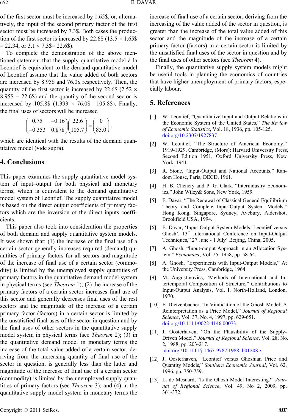

E. DAVAR 652
of thust be ined by 1.65$, terna-
tively, the input of the secoary factorrst
secased byth cases oduc-
tion ofcry 22.6$ (1 1.65$
22.3 7.3$= 22.6$)
spectively. Then, the
qu
4. Conclusions
demand quantitative
tief. The supply quantitative m
output coefficients of primary fac-
increafinal use of a certa sector, derivingrom the
increasing of the value added of the sector in question, is
greate the increase of total value add
sector ahe magnitude of the increase of a certain
primary factor (factors) in a certain sector is liited by
e first sector mcreasor, al
nd prim of the fi
tor must be incre 7.3$. Bothe pr
the first sector is in
4, or 3.1 eased b . 3.5  =To complete the demonstration of the above men-
tioned statement that the supply quantitative model à la
Leontief is equivalent to the demand quantitative model
of Leontief assume that the value added of both sectors
are increased by 8.95$ and 76.0$ re
antity of the first sector is increased by 22.6$ (2.52 
8.95$ = 22.6$) and the quantity of the second sector is
increased by 105.8$ (1.393  76.0$= 105.8$). Finally,
the final uses of sectors will be increased
0.750.1622.60
0.353 0.878105.785.0






.
which are identical with the results of the demand quan-
titative model (vide supra).
This paper examines the supply quantitative model sys-
tem of input–output for both physical and monetary
rms, which is equivalent to the te
model system of Leon
based on the direct odel is
tors which are the inversion of the direct inputs coeffi-
cients.
This paper also took into consideration the properties
of both demand and supply quantitative system models.
It was shown that: (1) the increase of the final use of a
certain sector generally increases required (demand) qu-
antities of primary factors for all sectors and magnitude
of the increase of final use of a certain sector (commo-
dity) is limited by the unemployed supply quantities of
primary factors in the quantitative demand model system
in physical terms (see Theorem 1); (2) the increase of the
primary factors of a certain sector increases final use of
this sector and generally decreases final uses of the rest
sectors and the magnitude of the increase of a certain
primary factor (factors) in a certain sector is limited by
the unsatisfied final uses of the sector in question and by
the final uses of other sectors in the quantitative supply
model system in physical terms (see Theorem 2); (3) in
the quantitative demand model in monetary terms the
increase of the total value added of a certain sector, de-
riving from the increasing quantity of final use of the
sector in question, is generally less than the latter and
magnitude of the increase of final use of a certain sector
(commodity) is limited by the unemployed supply quan-
tities of primary factors (see Theorem 3); and (4) in the
quantitative supply model system in monetary terms the
the unsatisfied final uses of the sector in question and by
the final uses of other sectors (see Theorem 4).
Finally, the quantitative supply system models might
be useful tools in planning the economics of countries
that have higher unemployment of primary factors, espe-
cially labour.
5. References
[1] W. Leontief, “Quantitative Input and Output Relations in
the Economic System of the United States,” The Review
of Economic Statistics, Vol. 18, 1936, pp. 105-125.
se of in f
r thanhe ted of this
nd tm
doi:org/10.2307/1927837
[2] W. Leontief, “The Structure of American Economy,”
1919-1929. Cambridge, (Mors): Harvard University Press,
Second Edition 1951, Oxford University Press, New
York, 1941.
[3] R. Stone, “Input-Output and National Accounts,” Ran-
.
and P. G. Clark, “Interindustry Econom-
ics,” John Wiley& Sons, New York, 1959.
hot,
dom House, Paris, DECD, 1961
4] H. B. Chenery[
[5] E. Davar, “The Renewal of Classical General Equilibrium
Theory and Complete Input-Output System Models,”
Hong Kong, Singapore, Sydney, Avebury, Alders
Brookfield USA, 1994.
[6] E. Davar, ‘Input-Output System Models: Leontief versus
Ghosh’, 13th International Conference on Input-Output
Techniques,” 27 June - 1 July’ Beijing, China, 2005.
[7] A. Ghosh, “Input-output Approach in an Allocation Sys-
tem,” Economica, Vol. 25, 1958, pp. 58-64.
[8] A. Ghosh, “Experiments with Input-Output Models,” At
the University Press, Cambridge, 1964.
[9] M. Augustinovics, ‘Methods of International and In-
tertemporal Composition of Structure,” Contributions to
Input-Output Analysis, Vol. I, North-Holland, London,
1970.
[10] E. Dietzenbacher, ‘In Vindication of the Ghosh Model: A
Reinterpretation as a Price Model,” Journal of Regional
Science, Vol. 37, No. 4, 1997, pp. 629-651.
doi:org/10.1111/0022-4146.00073
[11] J. Oosterhaven, “On the Plausibility of the Supply-
Driven Model,” Journal of Regional Science, Vol. 28, No.
208.x
2, 1988, pp. 203-217.
doi:org /10.1111/j.1467-9787.1988.tb01
esnard, “Is the Ghosh Model Interesting?” Jour-
[12] J. Oosterhaven, “Leontief versus Ghoshian Price and
Quantity Models,” Southern Economic Journal, Vol. 62,
1996, pp. 750-759.
[13] L. de M
nal of Regional Science, Vol. 49, No 2, 2009, pp.
361-372.

E. DAVAR653
, Wages, and
Economy
hoice of Technology,” Scien
[14] W. Leontief, ‘Technological Change, Prices
Rates of Return on Capital in the USA ,” In-
put-Output Economics, Second Edition, Oxford Univer-
sity Press, New York, 1986.
[15] W. Leontief, “The C
American, Vol. 252, No. 6, pp. 25-33, 1985. tific
doi:org/10.1038/scientificamerican0685-37
[16] E. Davar, “Input-Output in Mixed Measurements,” 13th
International Conference on Input-Output Techniques
, 2000.
w-Hill, New
Equilibrium,” Eco-
, no
21-25 August, Macerate, Italy
[17] R. Dorfman, “Samuelson, P. and R. Solow: Linear Pro-
gramming and Economic Analysis,” McGra
York, 1958.
[18] W. Leontief, “Input-Output Economics,” Oxford UP,
New York, 1966.
[19] E. Davar, “Input-Output and General
mic Systems Research, Vol. 1, No. 3, pp. 331-343,
1989.