Smart Grid and Renewable Energy
Vol.4 No.2(2013), Article ID:32183,6 pages DOI:10.4236/sgre.2013.42022
Very Short-Term Generating Power Forecasting for Wind Power Generators Based on Time Series Analysis
![]()
1University of the Ryukyus, Okinawa, Japan; 2Meidensha Corporation, Tokyo, Japan; 3Sungkyunkwan University, Suwon City, South Korea.
Email: yona@tec.u-ryukyu.ac.jp, b985542@tec.u-ryukyu.ac.jp, funabashi-t@mb.meidensha.co.jp, chkimskku@yahoo.com
Copyright © 2013 Atsushi Yona et al. This is an open access article distributed under the Creative Commons Attribution License, which permits unrestricted use, distribution, and reproduction in any medium, provided the original work is properly cited.
Received December 28th, 2012; revised January 28th, 2013; accepted February 5th, 2013
Keywords: Very Short-Term Ahead Forecasting; Wind Power Generation; Wind Speed Forecasting; Time Series Analysis
ABSTRACT
In recent years, there has been introduction of alternative energy sources such as wind energy. However, wind speed is not constant and wind power output is proportional to the cube of the wind speed. In order to control the power output for wind power generators as accurately as possible, a method of wind speed estimation is required. In this paper, a technique considers that wind speed in the order of 1 - 30 seconds is investigated in confirming the validity of the Auto Regressive model (AR), Kalman Filter (KF) and Neural Network (NN) to forecast wind speed. This paper compares the simulation results of the forecast wind speed for the power output forecast of wind power generator by using AR, KF and NN.
1. Introduction
Wind generators are rapidly gaining acceptance as some of the best alternative energy sources, and an alternative to conventional power generation. Especially due to decreasing cost of the wind generated power, it has the potential to compete with traditional power plants. However, wind speed is not constant and the power output of wind generators is proportional to the cube of the wind speed. The intermittent nature of wind makes the power output fluctuation of wind generator. In electric companies, wind speed forecasting is an important tool for utilizing the hybrid power systems with storage battery, wind generators, solar cells, etc. For example, the amount of energy stored in the battery is easily decided by forecast data. These decisions are beneficial for effective operation of hybrid power systems and consequently, their profitability depends on the technique utilized in the forecasting powers. Although the technique to forecast power output of wind generators based on wind speed prediction is regarded as an effective method in practical applications, it requires large meteorological data. In addition, although meteorological agencies or weather services will provide free data for prediction, the implementation of the above-mentioned techniques provide the order of several minutes data or hourly data. Since the data is mostly gathered over a wide area by prediction, it becomes rather difficult to determine the exact values for the order of several seconds at the installation area of a wind generator. Auto Regressive Model (AR) [1], Kalman Filter (KF) [2-4] and Neural Network (NN) [5-16] have been known that techniques are convenient in forecasting applications. It is possible to forecast wind speed by using only meteorological data. There is a valid argument: AR and KF are well known models for 1 - 3 time steps ahead forecasting. However the forecast result of using NN is usually case-by-case with the characteristic (stochastic appearance) of wind speed.
This paper describes very short-term ahead power output forecasting of wind generators based on wind speed forecasting. For the purpose of comparing the forecasting abilities of AR, KF and NN in this paper, all input data are based on the same condition. These models are constructed by using historical data on wind speed and tested for the target time. In addition, these data are observed at only one specific site. The power output of the wind generator is determined by the forecast wind speed data. The abilities of these models are confirmed by comparing the results in 1 - 30 seconds ahead forecasting.
2. Methodology and Application Model
The concept of the wind speed forecast technique is shown in Figure 1. In this paper, it is assumed that 1 to 30 seconds are forecast period of the wind forecasting. AR, KF and NN are constructed by making use of the historical data of 1 - 30 seconds at before 1-second. The idea is assumed that these models are constructed respectively in regard to the application of time series. It means the previous 30 seconds data reflect the trend of wind characteristic to forecast models with simple approach. After the wind speed forecasting, these three outputs are utilized for determination of power outputs of wind power generator. Explanation of AR, KF and NN are given below.
2.1. Auto Regressive Model
A common approach for modelling of time series is the AR model. The method of least-squares is applied in the estimation method of AR model. To apply the least squares method for time-varying AR model estimation, AR parameters are assumed to be time-invariant. If we want to obtain the forecast value , regression coefficient
  and residual error
  should be determined by:
 (1)
(1)
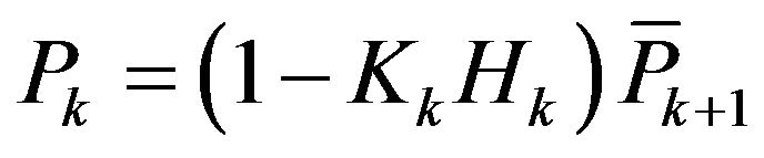
2.2. Kalman Filter
The Kalman filter is a recursive estimator. It means that only the estimated state from the previous time step and the current measurement are needed for the current state. The first task during update of measurement is to compute the Kalman gain . If estimated value
  and covariance matrix
  for estimate error are obtained,
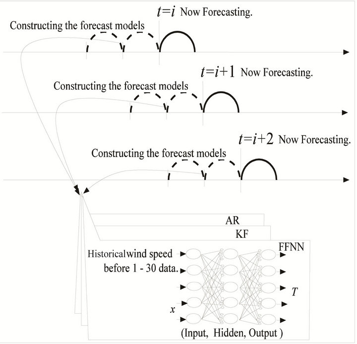
Figure 1. The concept of the forecast technique.
the next step is to measure the process to obtain observed value , and update the estimated value
  and covariance matrix
  for posteriori estimation. This process is represented by:
 (3)
(3)
 (4)
(4)
 (5)
(5)
where R is covariance for observation error, H is m × n matrix, which shows the relation between the state variable of a system and an observed value. 1 step-ahead estimation value  and covariance matrix
  for estimation errors are calculated by:
 (6)
(6)
 (7)
(7)
where Ak is n × n matrix, Bk is n × l matrix, Qk is covariance of process error,  will be update of zk after 2 steps ahead.
2.3. Neural Network
Figure 2 shows the Feed-forward Neural Network (FFNN), having l and m neurons in input layer and hidden layer respectively, and n neurons in output layer. These neurons are connected with a linear coupling, and x1 - xl are input data to NN. There are connection weights between each neuron. The output of the hidden neurons and output neurons are converted to nonlinear values by the sigmoid function. The sigmoid function is as follows:
 (8)
(8)
where, x is the input data.
Back Propagation (BP) method is adopted for training the NN. Generally, BP is explained as follows. To begin with, output of the hidden neuron is transmitted to the output neuron. Then the output of the output neuron is

Figure 2. Neural network.
compared with target signal, T, as shown in Figure 2. Finally, to minimize the mean square error margin, each connection weight and the output value of each neuron are changed in the direction of a straight line from output layer to input layer. In this paper, Levenberg-Marquardt algorithm [17] was adopted for training each connection weight of neurons. The “momentum” and “training coefficient” terms are parameters of training; momentum promotes training speed and acts rapidly by changing each connection weight of neurons. The training coefficient parameter has to be large; however, if it is too large, the network becomes unstable. It is desired that the mean square error margin of NN model should not be unstable. The authors determined these parameters by a trial-anderror method.
3. Simulation Results
This section shows the simulation results of wind speed forecasting. Analysis results of forecasting error are also described below. The wind speed is important parameter to know the forecasted power output of wind turbine. Because of the accuracy of the forecasted power output depends on characteristic of fluctuating power output and also wind speed.
3.1. Wind Speed Forecasting
Figure 3 shows the results of 10 sec ahead wind speed forecasting at the time t = 121 - 900 for observation (1-second intervals), and calculates the forecast error (MAE, mean absolute error) by using AR, KF and NN as shown in Figure 4. In the case of Figure 4, mean value of wind speed is 14.3265 m·s−1, and the variance is 3.6736 m·s−1. MAE is given as:
 (9)
(9)
where N is number of data,  is forecast value,
  is actual value, and k is forecast time. In the result of using AR, the forecast error (MAE) is 1.6169 m·s−1 in 10 sec ahead, while KF and NN cause 1.6120 m·s−1 and 1.6047 m·s−1, respectively. Figure 4 shows the calculated MAE of 1 - 30 ahead wind speed forecast. In wind speed forecasting, as forecast time lengthens, forecast error increases. This phenomenon appears prominently in the result shown in Figure 4. There are no differences in calculated results of MAE with AR model, KF and NN. But the forecast results of these models vary on a case-by-case basis with the characteristic (stochastic appearance) of wind speed. In the case of AR model, Figure 3(a) shows that the forecast result of 10 sec ahead wind speed is influenced by gradient between forecast time and before 10 sec wind speed. In the case of NN, Figure 3(b) shows that the result of 10 sec ahead wind
 (a)
(a)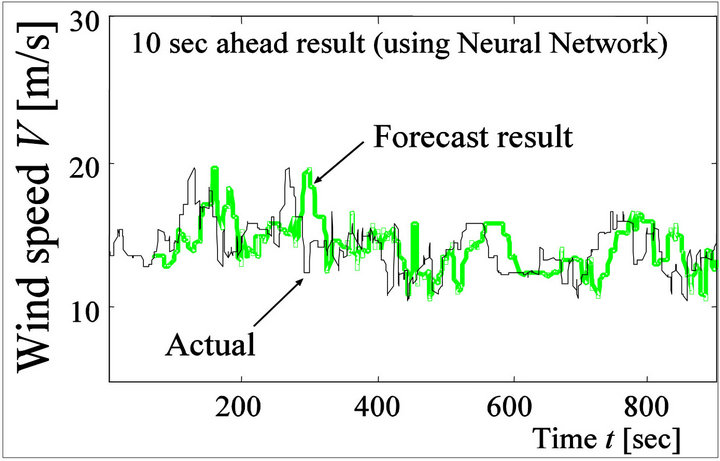 (b)
(b) (c)
(c)
Figure 3. Simulation result for 10 sec ahead wind speed forecasting. (a) The result for using auto regressive model; (b) The result for using neural network; (c) The result for using Kalman filter.
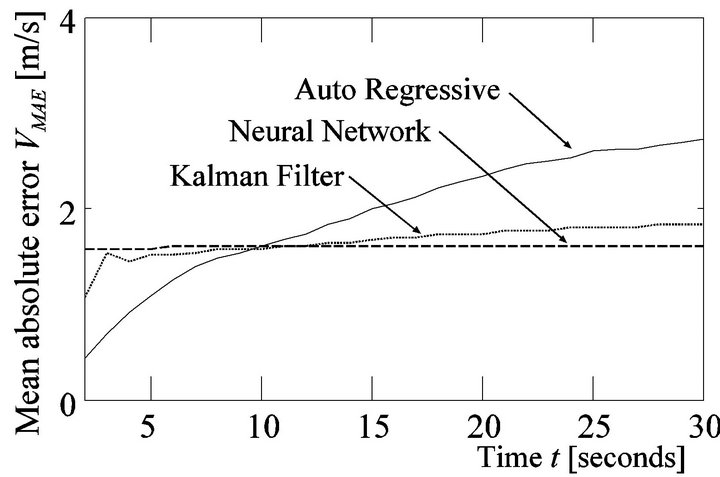
Figure 4. Mean absolute error VMAE (wind speed forecasting).
speed is influenced by before 1 - 30 seconds wind speed characteristic. In the case of KF, Figure 3(c) shows that the 10 sec ahead forecast result is similar to the result of using AR model, but the gradient between forecast time and before 10 sec wind speed have an insignificant effect on forecast result. In the simulation results of the forecasted wind speed, each of these models has its own merits and demerits as shown in Figure 3. But one of the criterions to decide the forecast performance of these models is described along with forecast time as shown in Figure 4.
3.2. Power Spectral of Wind Speed
Figure 5 shows the power spectral of wind speed at the time t = 121 - 900 s for observation in Figure 3. The power spectral (Van der Hoven model [18]) is as indicated below. The power spectral Syy(fk) for wind speed is an exponential-type Fourier transform Y(fk) calculated by observed wind speed y(t). Therefore, the power spectral Syy(fk) is represented by:
 (10)
(10)
where y(t) [m·s−1] is observed wind speed, Syy(fk) [m2·s−2] is the power spectral for wind speed, fk [Hz] is frequency, T [sec] is observation time, and N is the number of data. Fourier transform Y(fk) is obtained by:
 (11)
(11)
The power spectral density is usually represented by:
 (12)
(12)
Equation (10) supposes that wind speed has white noise properties, i.e., (distribution = 1, power spectral density = 1). Figure 5 shows that the power spectral of wind speed is low density at around 7 - 10 sec. Therefore, wind speed forecast errors of 7 - 10 sec ahead in Figures 3 and 4 are influenced by characteristic of wind speed for

Figure 5. Power spectral density of wind speed (Van der Hoven model).
the power spectral with low density.
4. Power Output of Wind Power Generator
After the wind speed forecasting, the authors determined the power output of wind power generator. In this paper, the point under discussion was put on wind speed forecasting. To confirm the validity of the proposed method, the authors determined the power output. It means that power output for wind generator can be forecast by using only wind speed data. The energy of the wind is kinetic energy, and kinetic energy of mass m and speed V is defined by 0.5 m·V2. Thus the wind power energy received by the swept area of the blades has the following equation:
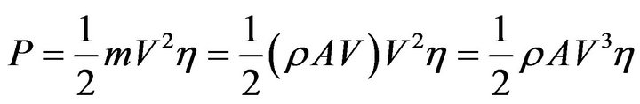 (13)
(13)
where m [kg] is mass, V [m·s−1] is wind speed, η [%] is efficiency coefficient, ρ is air density 1.225 kg·m3, and A [m2] is swept area of the blades [3]. Power output of a typical wind turbine is generated starting at “cut-in wind speed”, and not generated at over the “cut-out wind speed”. Rated wind speed is different in each type of wind turbine. Usually, cut in wind speed is 3 - 5 m·s−1, rated wind speed is 8 - 16 m·s−1, and cut out wind speed is 24 - 25 m·s−1 [19-21]. In this paper, power output of wind power generator is determined by parameters shown in Table 1 and Figure 6. As mentioned above, the
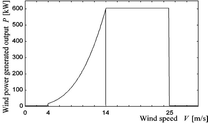
Figure 6. Power output curve of wind power generation system.
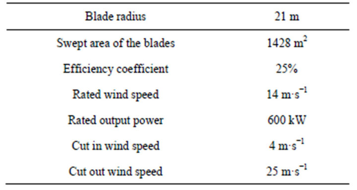
Table 1. Simulation parameters of tested wind power generator.
power output of wind power generator is determined by using only wind speed data.
Figure 7 shows the forecasting results of power output of wind power generator. The results of Figure 8 are
 (a)
(a) (b)
(b) (c)
(c)
Figure 7. Simulation result of 10 sec ahead forecasting power output for wind generator. (a) The result for using auto regressive model; (b) The result for using neural network; (c) The result for using Kalman filter.
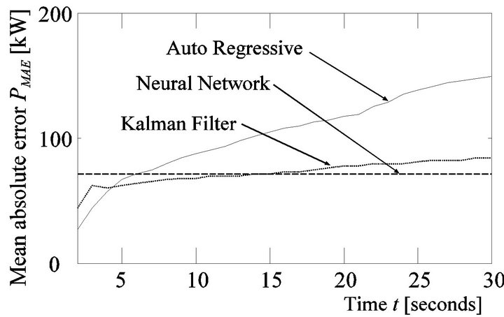
Figure 8. Mean absolute error PMAE (power output for wind generator).
calculated by wind speed forecasting shown in Figure 3. The calculated results of MAE with AR model, KF and NN are similar. But for the forecast result of the power output by using AR in Figure 7, the forecast error is 87.0152 kW in 10 sec ahead, while the results of KF and NN are 71.4639 kW and 68.7320 kW respectively. In fact, forecast error of power output increases by increasing forecast error of wind speed. Although our data sample is relatively small (representing only 900 wind speed data), adding data would further improve the model performance.
5. Conclusion
This paper shows the generating power forecasting of wind generators based on wind speed time series analysis by using AR, KF and NN. The constructed methods do not require complicated calculations due to wind speed data. At the time of wind speed forecasting, it is possible to shorten the calculation time by using historical wind speed data. The validity is confirmed by comparing forecasting results with AR, KF and NN. It is found that the proposed method shows good performance to forecast power output of wind generator. Simulation results lead to the conclusion that it is possible to build up the following hypotheses: if wind speed data are always available, the advantage of the proposed method in this paper is the ability to forecast and estimate sequences of seconds-scale power output for wind power generations from the wind speed only.
REFERENCES
- A. C. N. Salles, A. C. G. Melo and L. F. L. Legey, “Risk Analysis Methodologies for Financial Evaluation of Wind Energy Power Generation Projects in the Brazilian System,” 2004 International Conference on Probabilistic Methods Applied to Power Systems, 16 September 2004, pp. 457-462.
- D. E. Gustafson and W. H. Ledsham, “Applications of Estimation Theory to Inverse Problems in Meteorology,” 1978 IEEE Conference on Decision and Control Including the 17th Symposium on Adaptive Processes, Vol. 17, No. 1, 1978, pp. 405-412.
- L. Hui, K. L. Shi and P. G. McLaren, “Neural-NetworkBased Sensorless Maximum Wind Energy Capture with Compensated Power Coefficient,” IEEE Transactions on Industry Applications, Vol. 41, No. 6, 2005, pp. 1548- 1556. doi:10.1109/TIA.2005.858282
- G. Galanis, P. Louka, P. Katsafados, I. Pytharoulis and G. Kallos, “Applications of Kalman Filters Based on NonLinear Functions to Numerical Weather Predictions,” Annales Geophysicae, No. 24, 2006, pp. 1-10.
- M. A. Mohandes, S. Rehman and T. O. Halawani, “A Neural Networks Approach for Wind Speed Prediction,” Renewable Energy, Vol. 13, No. 3, 1998, pp. 345-354. doi:10.1016/S0960-1481(98)00001-9
- T. Toumiya, E. Sakaguchi, T. Tanaka and T. Suzuki, “Modeling of Wind Power Generating System with a Propeller Type Windmill by Neural Networks,” The Institute of Electrical Engineers of Japan, Vol. 118-B, No. 7-8, 1998, pp. 794-801. (in Japanese)
- Y. Kemmoku, H. Ishii, H. Takikawa, T. Kawamoto and T. Sakakibara, “Method of Forecasting Wind Velocity of Next Day Using Weather Data over Wide Area,” Journal of Japan Solar Energy Society, Vol. 27, No. 1, 2001, pp. 85-91. (in Japanese)
- P. Flores, A. Tapia and G. Tapia, “Application of a Control Algorithm for Wind Speed Prediction and Power Generation,” Renewable Energy, Vol. 30, No. 5, 2004, pp. 523-536.
- S. Kelouwani and K. Agbossou, “Nonlinear Model Identification of Wind Turbine with a Neural Network,” IEEE Transactions on Energy Conversion, Vol. 19, No. 3, 2004, pp. 607-612. doi:10.1109/TEC.2004.827715
- A. Oztopal, “Artificial Neural Network Approach to Spatial Estimation of Wind Velocity Data,” Energy Conversion and Management, Vol. 47, No. 4, 2006, pp. 395-406. doi:10.1016/j.enconman.2005.05.009
- J. L. Elman, “Finding Structure in Time,” Cognitive Science, Vol. 14, No. 2, 1990, pp. 179-211. doi:10.1207/s15516709cog1402_1
- J.-H. Li, A. N. Michel and W. Porod, “Analysis and Synthesis of a Class of Neural Networks: Linear Systems Operating on a Closed Hypercube,” IEEE Transactions on Circuits and Systems, Vol. 36, No. 11, 1989, pp. 1405- 1422. doi:10.1109/31.41297
- G. N. Kariniotakis, G. S. Stavrakakis and E. F. Nogaret, “Wind Power Forecasting Using Advanced Neural Networks Models,” IEEE Transactions on Energy Conversion, Vol. 11, No. 4, 1996, pp. 762-767. doi:10.1109/60.556376
- T. G. J. Barbounis, B. Thecharis, M. C. Alexiadis and P. S. Dokopoulos, “Long-Term Wind Speed and Power Forecasting Using Local Recurrent Neural Network Models,” IEEE Transactions on Energy Conversion, Vol. 21, No. 1, 2006, pp. 273-284. doi:10.1109/TEC.2005.847954
- Y. Kitamura and A. Matsuda, “Study on Raising Efficiency of Heat Accumulating Air Conditioning System Using Knowledge Processing Techniques,” Journal of Mitsubishi Research Institute, No. 36, 2000, pp. 31-51. (in Japanese)
- B. Kermanshahi, “Recurrent Neural Network for Forecasting Next 10 Years Loads of Nine Japanese Utilities,” Neurocomputing, Vol. 23, No. 1-3, 1998, pp. 125-133. doi:10.1016/S0925-2312(98)00073-3
- M. T. Hagan and M. B. Menhaj, “Training Feed-Forward Networks with the Marquardt Algorithm,” IEEE Transactions on Neural Networks, Vol. 5, No. 6, 1994, pp. 989- 993. doi:10.1109/72.329697
- V. D. Hoven, “Power Spectrum of Horizontal Wind Speed in the Frequency Range from 0.007 to 900 Cycles,” Journal of Meteorology, Vol. 14, No. 2, 1957, p. 160. doi:10.1175/1520-0469(1957)014<0160:PSOHWS>2.0.CO;2
- M. A. H. El-Sayed, “Substitution Potential of Wind Energy in Egypt,” Energy Policy, Vol. 30, No. 8, 2002, pp. 681-687. doi:10.1016/S0301-4215(02)00030-7
- M. A. Elhadidy and S. M. Shaahid, “Decentralized/StandAlone Hybrid Wind-Diesel Power Systems to Meet Residential Loads of Hot Coastal Regions,” Energy Conversion and Management, Vol. 46, No. 15-16, 2005, pp. 2501-2503. doi:10.1016/j.enconman.2004.11.010
- S. M. Shaahid, L. M. Al-Hadhrami and M. K. Rahman, “Economic Feasibility of Development of Wind Power Plants in Coastal Locations of Saudi Arabia—A Review,” Renewable and Sustainable Energy Reviews, Vol. 19, No. C, 2013, pp. 589-587. doi:10.1016/j.rser.2012.11.058