Journal of Transportation Technologies
Vol.05 No.04(2015), Article ID:60612,15 pages
10.4236/jtts.2015.54023
Design Optimization of an Oil-Air Catch Can Separation System
Anuar Abilgaziyev, Nurbol Nogerbek, Luis Rojas-Solórzano
Department of Mechanical Engineering, School of Engineering, Nazarbayev University, Astana, Kazakhstan
Email: a.abilgaziyev@gmail.com
Copyright © 2015 by authors and Scientific Research Publishing Inc.
This work is licensed under the Creative Commons Attribution International License (CC BY).
http://creativecommons.org/licenses/by/4.0/


Received 30 June 2015; accepted 24 October 2015; published 27 October 2015
ABSTRACT
The Positive Crankcase Ventilation (PCV) system in a car engine is designed to lower the pressure in the crankcase, which otherwise could lead to oil leaks and seal damage. The rotation of crankshaft in the crankcase causes the churn up of oil which conducts to occurrence of oil droplets which in turn may end in the PCV exhaust air intended to be re-injected in the engine admission. The oil catch can (OCC) is a device designed to trap these oil droplets, allowing the air to escape from the crankcase with the lowest content of oil as possible and thus, reducing the generation and emission of extra pollutants during the combustion of the air-fuel mixture. The main purpose of this paper is to optimize the design of a typical OCC used in many commercial cars by varying the length of its inner tube and the relative position of the outlet from radial to tangential fitting to the can body. For this purpose, CFD parametric analysis is performed to compute a one-way coupled Lagrangian-Eulerian two-phase flow simulation of the engine oil droplets driven by the air flow stream running through the device. The study was performed using the finite volume method with second-order spatial discretization scheme on governing equations in the Solid Works-EFD CFD platform. The turbulence was modelled using the k-ɛ model with wall functions. Numerical results have proved that maximum efficiency is obtained for the longest inner tube and the tangential position of the outlet; however, it is recommended further investigation to assess the potential erosion on the bottom of the can under such a design configuration.
Keywords:
CFD, Oil Catch Can, Positive Crankcase Ventilation, Motor Oil Droplets, Mesh Refinement, Two-Phase Flow, Lagrangian-Eulerian

1. Introduction
Manufacturers of motor vehicles design their products in accordance with external factors such as government and industry standards. These standards are related to aspects such as safety, performance, price through taxes and the most important to this research: emissions.
In the operation of an internal combustion engine, the crankshaft and the connecting rod act as a blender mixing the air and lubricating oil into a mist. In the 4-stroke process, the piston is forced down by the ignition of a mixture of compressed air and fuel that takes place inside the combustion chamber. The pumping action from the pistons pressurizes the crankcase, thus further mixing the air and oil. At the same time, a small amount of that ignited mixture leaks through the piston ring seals and ends up in the crankcase. This leakage is often mentioned as “blow-by” (see Figure 1 and Figure 2). In addition to the air-fuel mixture, there exists a large possibility of appearance of condensation and oil droplets [1] .

Figure 1. Schematic diagram of PCV system [2] .
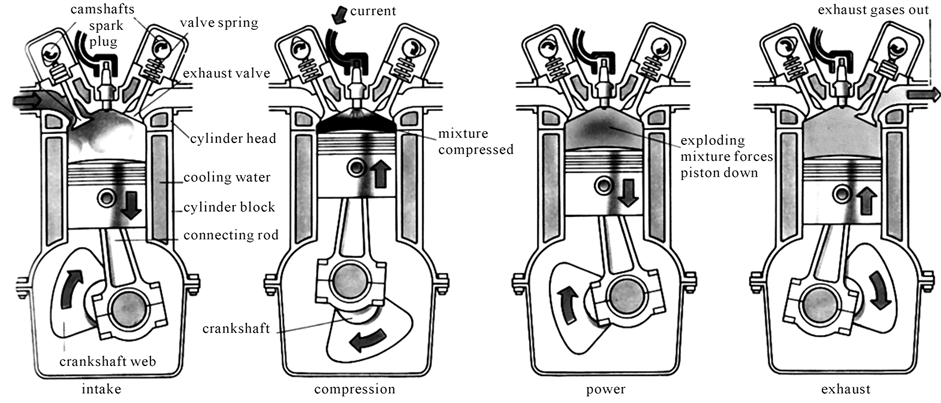
Figure 2. Schematic diagram 4-stroke engine process [5] .
This mixture of oil mist and hydrocarbons needs to be released and vented from the crankcase; otherwise a positive pressure will occur due to expansion, caused by heating of gases. Thus, gas-droplets mixture pressure inside the crankcase becomes higher than atmospheric pressure and if not taken care of, the mixture may diffuse onto the crankcase oil, contaminating it or else, it could return back to the intake manifold. In order to avoid or minimize this potential issue, engines are regularly equipped with breathers that would allow excess of crankcase pressure to be vented. However, the damage from not eliminating all gases out results in a reduced life of engine. In the end of 1950s, General Motors started to investigate the relationship between the hydrocarbons from gasoline engines and the environment (Filter Manufacturers Council, n.d.). Thus, the Positive Crankcase Ventilation (PCV) was developed and integrated to their cars by 1963 [3] .
According to Ding [4] , the main function of the PCV is to extract the mixture of gas-droplets from the crankcase by drawing fresh clean air in. The mechanism of operation is simple: air passes through the oil drain back passages to the crankcase below, displacing the dirty air-oil mist and hydrocarbons to the PCV valve. However, the PCV system is not perfect and it allows some of the oil mist back into the intake manifold, which will increase the level of carbon solids and reduce the octane level of the combustion fuel. For instance, for boosted setup with turbo and supercharger, the breather/PCV will not capture some of oil droplets. Thus, some of these oil droplets will recirculate from the intake to intercooler again and again. It will lead to reduction of heat exchange efficiency, since fume with oil droplets will coat the inside of the intercooler with oil. In addition, there exist other uncontrolled related issues such as the detonation or “knock” that occurs when oil is introduced into the combustion chamber triggering the action of the knock sensors pick-up and pull timing to protect the engine from damage, and thus reducing power. Another result is the carbon build-up on the valves and piston tops, which also results in decreased performance and less efficient performance. The main purpose of separating oil catch can (OCC) is to trap and remove these oil droplets from the gases before they will continue on through the intake and get burnt and consumed. Therefore, the OCC is placed in the PCV system, between PCV valve and intake manifold [6] .
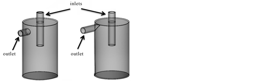
The OCCs are usually devised as an aftermarket device. The reason of it is that cars that need the separator come with individual built-in ones and not all cars necessarily need them. Thus, the only way OCCs could be publicly evaluated is by the amount of after-use oil found in the reservoir after a period of time of operation since the last oil change to the engine. The designs of OCCs in the market vary from a simple empty container with two pots to complex ones filled with some filters (see Figure 3). Therefore, this paper aims to obtain the most efficient design of an OCC by making some design modifications, ranging from the most common existing unit, with radial outlet, to a unit with fully tangential exit, depicted in Figure 4(a) and Figure 4(b), respectively.

Figure 3. Schematic diagram of the oil catch can [7] .
 (a) (b)
Figure 4. Physical generic CAD model of the OCCs. (a) Radial outlet; (b) Tangential outlet.
The independent parameters to be varied in the optimization process are the length of inner tube and the relative position of outlet pipe respect to can axis. The main hypothesis behind the use of those parameters is that these are simple changes that could be implemented with low expenses and would affect the travel-time of droplets and the exposure to surface contact which should portray an optimal configuration to maximize oil retention by the device.
The analysis here presented is based on CFD tools using a Lagrangian-Eulerian framework with one-direction coupling between phases, assuming the low volume fraction of the droplets compared to the airflow. Following a design of experiments approach with sampling of scenarios and construction of a surrogate model, the final optimal design is obtained based on the maximization of the collection efficiency, used as objective function.
The next sections are devoted to the following stages of the CFD study:
・ Prescription of governing equations and respective boundary conditions.
・ Description of verification of the discretization or Mesh Sensitivity Analysis.
・ Validation of the numerical tool (SolidWorks-EFD solver and physical models).
・ Preliminary results based on the analysis of the performance of most popular Oil Catch Can currently in the market.
・ Parametric study varying the input variables of interest in the optimization to validate the hypothesis.
・ Analysis and discussion, and concluding remarks.
2. Background
Nowadays, with the development of manufacturing industry, the fabrication of OCCs has also evolved and there exist various designs of cans [8] . For instance, some cans have pretty simple designs that consist of simple empty housing, inlet and outlet tube. In-deep background research of catch can was conducted and it was found that most companies use two main approaches for catch can design. The basic design is a simple can with hoses attached [8] . The more advanced designs include internal baffling, which provides more surface area for the oil to be collected, e.g. baffled OCC made by Mishimoto [9] . Though both of these approaches work, the simpler design is much less efficient than the complex unit.
One of the most popular companies manufacturing the OCCs is Mishimoto [9] . According to the Mishimoto Technical Specs [9] , their aim is to design a high-end oil/air separator that is universal and can be installed in any vehicle. At the same time Mishimoto engineers pursue a design with exceptional functionality and still looking aesthetically pleasing. Unfortunately, they did not publish the official results of their research, but indicate in their company’s web site that they created a new MMBCC-UNI model that claims to be the most effective oil catch can today on the market. However it should be understood that different motor vehicles have different type of engines and, therefore, each company manufacturing oil catch cans creates its own design for a specific type of engine or specific car make.
Thus, the design that was used as a base case in this work was based on the design that according to Mishimoto Technical Specs [9] is the most efficient and universal currently in the market. Since the goal of this paper is to develop a design optimization of the geometry of the oil catch can, the device was simplified and none of regular inner filters were included, but instead the numerical model will artificially capture all droplets hitting the can walls, as if they were naturally attached and drained out.
3. Numerical Model Set-Up
The OCC models, with inlet on the top part and outlet with two positions on the top part of the cylinder, are shown in Figure 4.
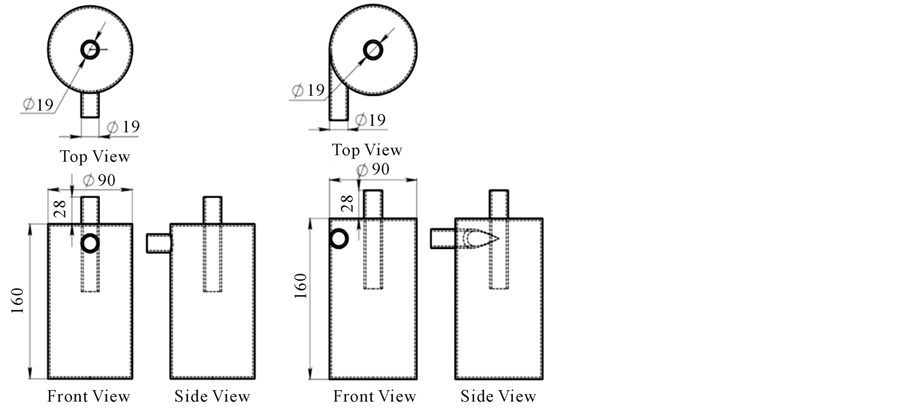
As it was mentioned before, all parameters of the can were taken from one of the most efficient and universal OCCs that are designed by Mishimoto Company. The CAD drawings with dimensions of the two main models of OCC, according to exit pipe, are shown in Figure 5.
Thus, two parameters, the length of inner tube from top to bottom and the position of the outlet, were taken into account for the analysis. The length of the inner tube is represented by X variable (the range is [30; 130] mm), whereas the position of the outer tube is Y (the range is [0, 35.5] mm) (see Figure 6).
 (a) (b)
Figure 5. Schematic multi-view drawings of the oil catch can with two critical types of outlet tube. (a) Radial outlet; (b) Tangential outlet.
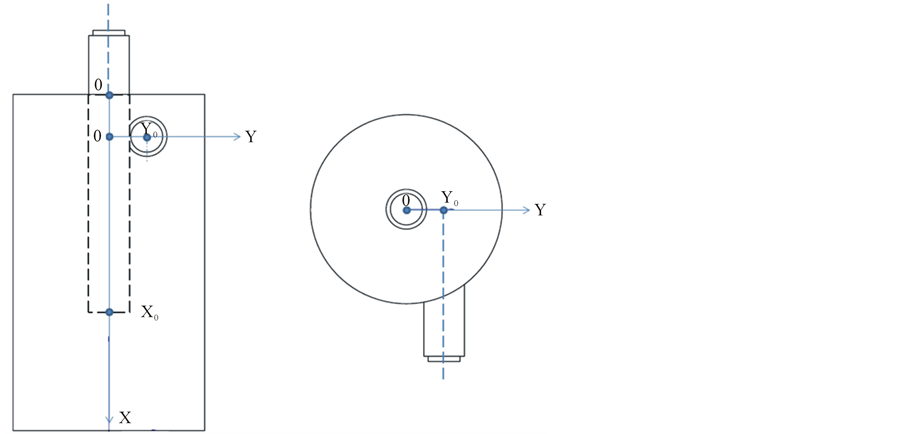
Figure 6. Demonstrating figure of Xo and Yo distances.
3.1. Mathematical Model
The setup of the mathematical model is performed using the CFD workbench SolidWorks-FloEFD (SW-FloEFD) v.2013-14. The main premises are: steady state, Newtonian fluid, compressible and turbulent flow. Therefore, the following favré-averaged governing equations and boundary conditions were prescribed: (a) mass conservation; (b) Navier-Stokes (momentum conservation) equations; (c) energy conservation; (d) constitutive relations between p, T and H; and (f) k-ɛ turbulence model with wall functions. These equations for the air are shown as follows:
 (2.1)
(2.1)
 (2.2)
(2.2)
with:
 (2.3)
(2.3)
(Newtonian fluid constitutive equation to turn the momentum equations into Navier-Stokes equations).
 (2.4)
(2.4)
(Boussinesq’s assumption for the Reynolds-stress) where, δij is the Kronecker delta function, μ is the dynamic viscosity, μt is the turbulent eddy viscosity and k is the specific turbulent kinetic energy.
The energy transport equation for the fluid in terms of the enthalpy:

 (2.5)
(2.5)
The Ideal Gas state equation is prescribed to compute the air density as a function of pressure and temperature:

with:
 (2.6)
(2.6)
For the oil droplets trajectories within the fluid (air), the solver assumes spherical liquid particles (droplets) in a steady-state air flow field. Only fluid-to-particle interaction is allowed, thus the model is limited to dilute particles only, which is in general valid for bulk mass ratio of particles to fluid of less than 20% - 30%, as in this case. The particles drag is calculated using Henderson’s formula [10] , which accounts for laminar/transitional/ turbulent flow regimes and temperature difference between particles and carrier fluid. The particle/fluid heat transfer is computed according to Carlson and Hoglund [11] formula and since each particle mass is assumed constant, the size may change accordingly, as they are cooled or heated by the surrounding air. The gravity is included in the analysis and the walls are treated as adiabatic with full absorption of any particle that hits them.
The additional k-ɛ transport equations for the specific turbulent kinetic energy and dissipation respectively are:
 (2.7)
(2.7)
 (2.8)
(2.8)
where, the source terms are defined as:
 (2.9)
(2.9)
 (2.10)
where, PB represents the turbulent production due to buoyancy forces and is given by:
 (2.11)
with gi = (gx, gy, gz) the gravity vector, the constant σB = 0.9 and constant CB = 1 when PB > 0, and 0 otherwise. Whereas:
 (2.12)
The constants Cμ, Cɛ1, Cɛ2, σk, σɛ are obtained from typical fitting experiments as:
 (2.13)
The diffusive heat flux is defined as:
 (2.14)
with the constant σc = 0.9, Pr is the Prandtl number and α is the thermal diffusivity.
And the relation between k, ɛ and μt is given by:
 (2.15)
and fμ is a turbulence damping factor to consider the laminar-turbulent transition as a function of distance from the wall, defined by the expression:
 (2.16)
where:
 (2.17)
and y is the distance from the wall.
3.2. Boundary Conditions
The following boundary conditions are prescribed on the governing equations:
・ Inlet air volume flow rate is 5 cfm (~2.35 × 10⁻³ m3/s) [12] .
・ Inlet static pressure and temperature are 7 bar and 700˚C, respectively. Since inlet flow was obtained from the combustion chamber with high rpm motor, the inlet air is assumed with same pressure and temperature of average parameters (pressure and temperature) of the combustion chamber. The average values are obtained from the graph shown in Figure 7.
・ Outlet static pressure and temperature are 1 bar and 20˚C, respectively. These values are obtained from the graph of pressure and temperature against crank angle in the combustion chamber (Figure 7). It is assumed that the outlet has the thermodynamic conditions as the air in the intake stroke (approximately in the range [−270, −90] degrees of crank angle) since other end of blow-by-gas line is connected to intake air for re- combustion (Figure 8).
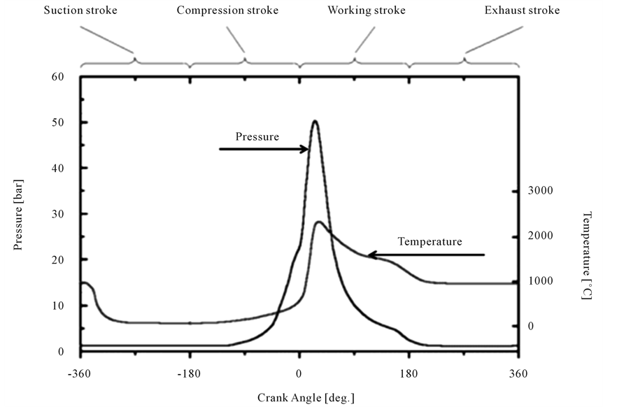
Figure 7. Pressure and temperature behaviour in the combustion chamber of a 4-stroke engine [13] .

Figure 8. Schematic diagram of the principle of how OCC works [14] .
The properties for the motor oil are listed below:
・ Density (ρ) = 895 kg/m3 [15] .
・ Kinematic viscosity (ν) = 1.01 × 10⁻⁵ m2/s (= 10.1 cSt) [15] .
・ Dynamic viscosity (μ) = 0.01 Pa・s (found by the formula μ = ρν using previous parameters).
・ Specific heat = 1900 J/(kg・K) [16] .
・ Thermal conductivity = 0.2 W/(m・K) [16] .
The mass flow rate of the oil is 2.89 × 10⁻⁷ kg/s. The value is estimated by knowing the volume of the oil caught when a car is driven for approximately 2400 m (1500 miles) from a video in YouTube Channel: newagemuscle 2010 ss [17] . Taking average velocity of the car as 30 km/h [18] , we can obtain approximate volume flow rate of the oil to finally get the mass flow rate of oil flowing into the catch can, which as expected, is much smaller than the mass flow of air as expected. For the modelling, the sizes of droplets are so small that the droplets of the oil are considered as perfect spheres. For the simulation, the diameter of the droplets is taken as 1.5 µm [19] .
The inner wall is set to absorb oil droplets hitting it. Some particles will not be caught by the wall which will leave the can with the air stream. Thus, the lower the number of particles leaving the can, the higher the OCC efficiency. Hence, the efficiency of the OCC is calculated by the formula:

where Ni is the number of droplets at inlet and No is the number of droplets at outlet. Assuming the velocity of droplets at inlet is equivalent to the velocity of the air, number of droplets at inlet would be approximately 200 for this study.
3.3. Discretization and Mesh Sensitivity Analysis
In order to ensure proper and acceptable accuracy of the results, the discretization mesh has to undergo a Mesh Sensitivity Analysis (MSA), in which density of cells is gradually increased, with special attention to region of largest gradients, and the solution must be re-assessed until results demonstrate sufficient independence on grid size.
For the MSA, the catch can model with Y = 35.5 mm and X = 130 mm specifications is selected, since this corresponds to the most critical configuration due to the expected helical motion of the air stream carrying the droplets.
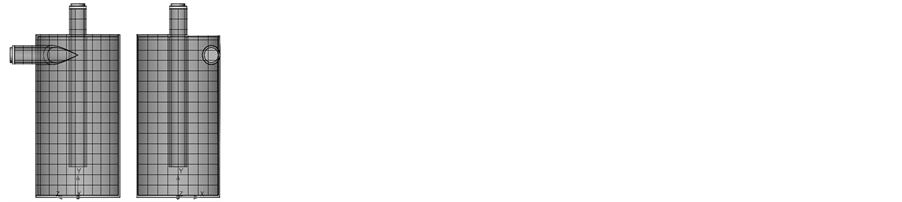
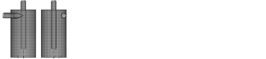
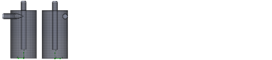
The discretization of the geometry was performed according to the following mesh parameters: initial coarse mesh with total number of cells equal to 27,381. Mesh refined by the range of 50% - 65% with total of 43,725, and this was repeated until results converged satisfactorily. The mesh refinement process stopped when the difference in overall pressure drop between consecutive meshes was less than 1%, which occurred for mesh with 112,525 cells. This level of error was acceptable given the complexity of the two-phase flow model and its difficulty to obtain full convergence. The main generated computational grids during the MSA are presented in Figure 9 and results are summarised in Table 1.
The set of governing equations are discretized and solved using the finite volume (FV) method on a spatially rectangular computational mesh refined locally at the solid/fluid interfaces and in specified fluid regions where high gradients are expected. The FV method grants a conservative discretization of the governing equations,
 (a) (b) (c) (d)
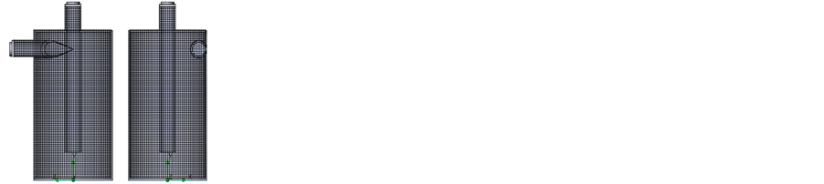
Figure 9. Side and front views for meshes during MSA. (a) 27,381 cells; (b) 43,725 cells; (c) 71,405 cells; (d) 112,525 cells.

Table 1. Summary of MSA.
with spatial derivatives (fluxes) approximated with second-order upwind on the implicitly treated modified Leonard’s QUICK (Quadratic Upstream Interpolation of Convective Kinematics) [20] and a Total Variation Diminishing (TVD) method [21] .
An operator-splitting technique [22] -[24] to efficiently resolve the problem of pressure-velocity decoupling, following a SIMPLE/like approach [25] is used.
The resulting linearised algebraic system of equations is solved by iteration on the LU-factorization preconditioned matrix using the generalized conjugate gradient method [26] . The stop criterion is reached when the difference between consecutive iterations for global mass flow conservation is met at less than 0.001% of inlet flow rate (~2.82 × 10⁻⁸ kg/s).
3.4. Computational Resource
The simulations were carried out using a PC with CPU Intel(R) Core(TM) i7-3517U @ 1.90 GHz, 2.40 GHz and 8.00 GB RAM characteristics. The time taken for every simulation with the finally chosen mesh to fully convergence starting from previously converged results in coarser mesh was approximately 1 hour.
3.5. Validation of SW-FloEFD Model
Transportation of small particles and their trajectories in uniform flows were already validated for SW-FloEFD [27] . Two different type of validations were presented: (a) trajectories of massless particles initially injected perpendicular to uniform flow are numerically predicted in excellent agreement with theoretical trajectories; (b) trajectories of the particles in similar conditions but including gravitational effects are also numerically calculated in very good agreement with theoretical results. Detailed information may be found in the references.
Moreover, SW-FloEFD has been validated for laminar and turbulent flows in pipes [28] . The longitudinal pressure gradient along a pipe and the fluid velocity profile at the pipe exit at various Re were calculated in excellent agreement with theoretical solution for laminar flow and experimental data for turbulent regime. Further details may be found in the references.
4. Methodology
The optimization proceeded with the independent two parameters Xo and Yo already described, using a second order two-variable “multivariate nonlinear regression analysis” (MNRA) in the form of quadratic equation with two variables. The physical ranges were Xo: [30, 130] mm and Yo: [0, 35.5] mm, respectively, but were normalised as (x, y) with range of [0, 1] each one to facilitate the manipulation of data and minimise round-off errors during the operations. Therefore, the objective function is described by  where f(x, y) is the OCC efficiency.
At first, the second-order equation, representing a surrogate of the real complex model described by governing equations and boundary conditions, is found by the regression analysis with 9 input pair of data points. After that, the critical point (i.e. the highest efficiency) is found by maximizing the surrogate function. Afterwards, a random pair of data points is chosen and its efficiency is evaluated using CFD simulation. Once the result is obtained, this new point is integrated to the MNRA and a new surrogate is derived. From this new surrogate function, the critical point is found and its efficiency (maximum) is compared to the maximum from previous surrogate (iteration). If the comparison is not satisfactory, a new pair of data points is randomly drawn and the process is repeated until the maxima between consecutive iteration differ less than ~1%.
5. Numerical Results
The initial 9 chosen different OCC’s configuration are simulated and the efficiencies were obtained as shown in Table 2.
Then, MNRA led to 6 coefficients of the surrogate function. All results are shown in Table 3 for 5 consecutive iterations. Four random points with respective efficiency for each, as obtained are shown in Table 4, including the points with maximum efficiency.
On the 5th iteration, the error is reduced to 1.23%. The best fit equation of the efficiency behaviour is shown below:

The final critical point for maximum efficiency is (x, y) = (0.8369, 0.9243), which is equivalent to (Xo, Yo) = (113.69, 32.8127) in mm. At this point, the efficiency is 0.69 (69%).
After this numerical analysis, it is observed that when x and y are approximately in the range of [0.5, 1], higher efficiency of the OCC is obtained (see Figure 10).
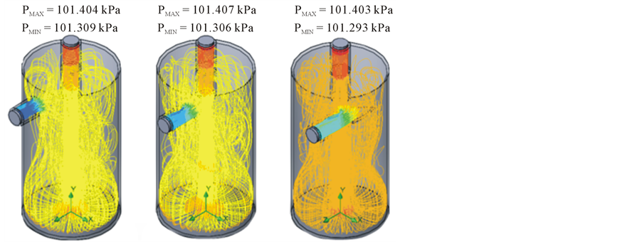
Trajectory lines of particles are shown in Figure A1 (see Appendix I). Colours on trajectory lines depict the fluid pressure at each location along the lines, for reference purposes.
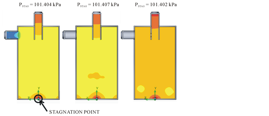
Regarding to the length of the inner tube, it is observed that the pressure at the stagnation (see Figure A2(a), Appendix II) bottom dramatically increases with increase of the inner tube’s length since the jet impinges more directly and less lateral diffusion is permitted (Figure A2). It is also noticed how the tangential outlet permits a more ordered exhaust and therefore the velocity recovery as the flow approaches the exit is more gradual than for the radial exhaust for all inner tube lengths. Figure A2 shows the positive relationship between the inner tube’s length which, when enlarged, increases the absorption of oil droplets and efficiency of the OCC.
Table 2. Efficiency results of initial 9 points.
Table 3. Obtained coefficients of the quadratic equation.
Table 4. Results from trial equation.
Moreover, the results show that the efficiency, when the outlet is located close to tangent (i.e., largest y-value) to the can, would be higher than the conventional radial outlet can (y = 0 mm). The main reason is that in the tangen- tial outlets the particle trajectories have a rotational motion that permits to have longer time in potential contact with the wall or filters, and therefore it increases the possibility to capture more droplets by the filters or walls.
6. Sentivity of CFD Results
In order to assess how sensible are the numerical results to changes in boundary conditions that may have an intrinsic level of uncertainty, i.e., mass flowrate of droplets and number of droplets injected through the inlet stream, a final sensitivity assessment was performed. The configuration Xo and Yo at their intermediate value, i.e., [80, 17.5] mm was used for this purpose, comparing the efficiency of the base case conditions, i.e., 200 droplets and 2.89 × 10⁻⁷ kg/s of oil at inlet flow stream with the efficiency obtained for ±20% variations of both parameters. Table 5 shows the comparison.
Results of sensitivity analysis demonstrate the low dependence of the predicted numerical results with respect to a moderately larger or smaller number of droplets and mass flowrate through the inlet of the catch can. In
Table 5. Sensitivity of CFD results to droplets flow and size.
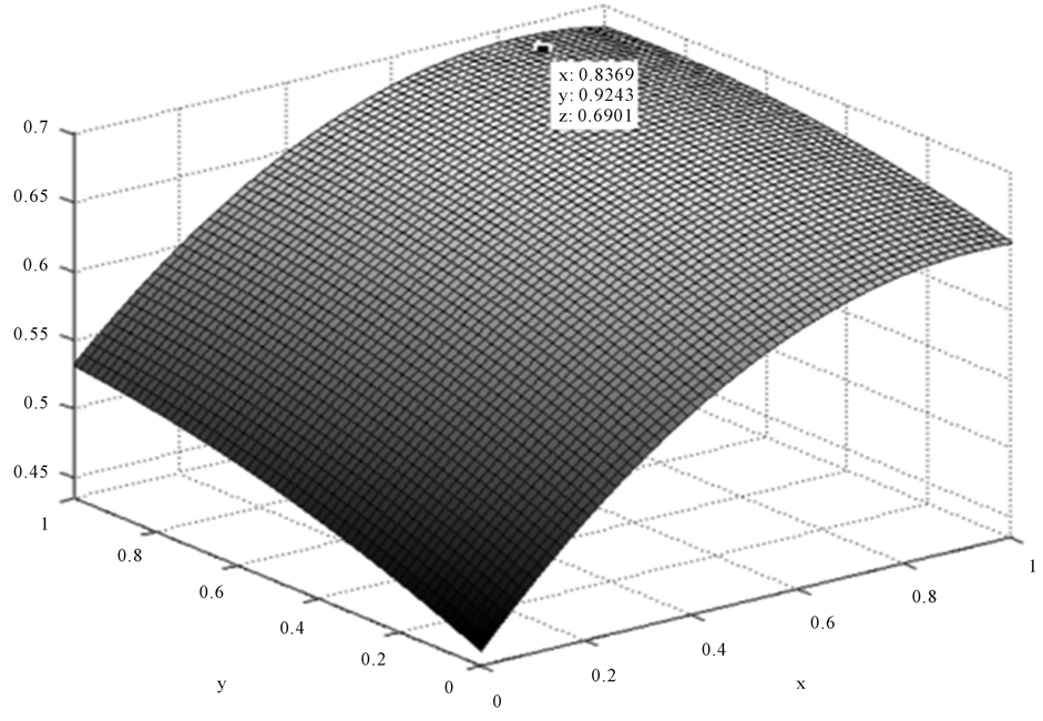
Figure 10. Efficiency against height of inner tube (x) and position of the outlet tube (y).
essence, the larger the amount of oil introduced in the catch can, the larger the amount of oil captured, at least within the 20% range variation around the level of oil inflow used for the optimization analysis. For that range variation, indeed, the predicted efficiency did not change more than 1%, supporting the robustness of the design obtained from the optimization analysis.
7. Concluding Remarks
A classical design of OCC is here optimized using CFD techniques and a Multivariable Nonlinear Regression Analysis to build a surrogate function which afterwards permits to maximize the droplet collection efficiency based on length of inner tube, x, and location of outlet tube respect to radial position, y. The results show that the efficiency is higher when the outlet is located tangentially to the can. Moreover, it is observed that more droplets are absorbed when the longer-inner-tube configuration is used, reaffirming the fact that the flow has more direct impact on walls and particles are more likely to get captured by walls leading again to a higher efficiency. However, caution should be paid since the closer the inner tube is to the OCC bottom, the larger the potential erosion and abrasion might be. This particular potentially negative effect deserves further study.
Acknowledgements
We would like to acknowledge the support of the School of Engineering at Nazarbayev University for giving us open access to its computer laboratory.
Cite this paper
AnuarAbilgaziyev,NurbolNogerbek,LuisRojas-Solórzano, (2015) Design Optimization of an Oil-Air Catch Can Separation System. Journal of Transportation Technologies,05,247-262. doi: 10.4236/jtts.2015.54023
References
- 1. Digsy (2005) Blow-By Breather Systems—Part One. [Online].
http://www.106rallye.co.uk/members/dynofiend/breathersystems.pdf - 2. AutoZone (n.d.) Schematic of the Positive Crankshaft Ventilation (PCV) System Air Flow in V6 and V8 Engines. [Online].
http://www.autozone.com/repairinfo/repairguide/repairGuideContent.jsp?pageId=0900c1528007db66 - 3. Filter Manufactures Council (n.d.) Positive Crankcase Ventilation. Technical Bulletin 94-2R1, Motor & Equipment Manufacturers Association, Washington DC. [Online].
http://www.baldwinfilter.com/literature/english/10%20TSB's/94-2R1.pdf - 4. Ding, G. (2011) Study on Extenics Information Fusion Method. International Journal of Engineering and Manufacturing, 1, 13-19.
http://dx.doi.org/10.5815/ijem.2011.01.03 - 5. Bhatt, E.V. (2013) 4-Stroke Engine. [Online].
http://www.makingdifferent.com/2-stroke-engine-and-4-stroke-engine/ - 6. Bolduc, J., Wentworth, F., Matthew, D. and Mackenzie, D. (2013) Oil-Air Vapor Separator. Capstone Project, University of Maine, Orono.
- 7. Bowman, C. (n.d.) 1999-2004 Mustang Catch Can Uses & Explanations. [Online].
http://www.americanmuscle.com/94-catch-me-if-you-can-99-04-mustangs.html - 8. Michael, J. (2013) Oil Catch Cans—What You Should Know—How They Work. The Torque Post. [Online]. https://torquepost.wordpress.com/2013/05/06/oil-catch-cans-what-you-should-know-how-the-work
- 9. Mishimoto (2013) Mishimoto Baffled Oil Catch Can. Technical Spec, Mishimoto Research and Development, New Castle. [Online].
http://www.mishimoto.com/mishimoto-baffled-oil-catch-can.html - 10. Henderson, C.B. (1976) Drag Coefficients of Spheres in Continuum and Rarefied Flows. AIAA Journal, 14, 707-708.
http://dx.doi.org/10.2514/3.61409 - 11. Carlson, D.J. and Hoglund, R.F. (1964) Particle Drag and Heat Transfer in Rocket Nozzles. AIAA Journal, 2, 1980-1984.
http://dx.doi.org/10.2514/3.2714 - 12. Vann, D.L. (1997) Crankcase Breating. [Online]
http://nortonownersclub.org/support/technical-support-commando/crankcase-breathing - 13. Ha, D. (2015) Pressure and Temperature Behavior in the Combustion Chamber of a 4-Stroke Engine. [Online]
http://www-mat.ee.tu-berlin.de/research/sic_sens/sic_sen3.htm - 14. Oil Catch Cans. What Are PCV Oil Catch Cans? Accessed on 16 April 2014.
http://oilcatchcan.com/ - 15. Nabi, N., Akhter, S. and Rahman, A. (2013) Waste Transformer Oil as an Alternative Fuel for Diesel Engine. Procedia Engineering, 56, 401-406.
http://dx.doi.org/10.1016/j.proeng.2013.03.139 - 16. Lam, S.S., Russell, A.D., Lee, C.L., Lam, S.K. and Chase, H.A. (2012) Production of Hydrogen and Light Hydrocarbons as a Potential Gaseous Fuel from Microwave-Heated Pyrolysis of Waste Automotive Engine Oil. International Journal of Hydrogen Energy, 30, 5011-5021.
http://www.sciencedirect.com
http://dx.doi.org/10.1016/j.ijhydene.2011.12.016 - 17. Newagemuscle2010ss (2014) Elite Engineering Catch Can. Results @ 1500 Miles. [Online Video] https://www.youtube.com/watch?v=JHol59_IeV4
- 18. Guilford, G. (2014) A Big Reason Beijing Is Polluted: The Average Car Goes 7.5 Miles Per Hour. Quartz. [Online]
http://qz.com/163178/a-big-reason-beijing-is-polluted-the-average-car-goes-7-5-miles-per-hour/ - 19. Smith, B.J. and Holness, M.H. (2005) Oil Mist Detection in the Atmosphere of the Machine Rooms. Marine Propulsion Conference. Bilbao, January 2005.
http://www.oilmist.com/bilbao-paper.pdf - 20. Roache, P.J. (1998) Technical Reference of Computational Fluid Dynamics. Hermosa Publishers, Albuquerque.
- 21. Hirsch, C. (1988) Numerical Computation of Internal and External Flows. John Wiley and Sons, Chichester.
- 22. Glowinski, R. and Tallec, P.L. (1989) Augmented Lagrangian Methods and Operator-Splitting Methods in Nonlinear Mechanics. SIAM, Philadelphia.
- 23. Marchuk, G.I. (1982) Methods of Numerical Mathematics. Springer-Verlag, Berlin.
- 24. Samarskii, A.A. (1989) Theory of Difference Schemes. Nauka, Moscow. (In Russian)
- 25. Patankar, S.V. (1980) Numerical Heat Transfer and Fluid Flow. Hemisphere, Washington DC.
- 26. Saad, Y. (1996) Iterative Methods for Sparse Linear Systems. PWS Publishing Company, Boston.
- 27. Dassault Systemes (2013) Technical Reference. SolidWorks Flow Simulation 2013. (2-82-2-88).
- 28. Dassault Systemes (2013) Technical Reference. SolidWorks Flow Simulation 2013. (2-17-2-22).
Nomenclatures
Cb: constant of the turbulent model
fµ: turbulence damping factor
gi: gravity vector
h: enthalpy
k: specific turbulent kinetic energy
p: static pressure
Pr: Prandtl number
R: specific gas constant
Si: gravity force per unit volume
T: static temperature
t: time
ui, uj, uk: velocity components in x, y and z directions, respectively
α: thermal diffusivity
γ: specific ratio
βij: Kronecker’s delta function
ε: turbulent energy dissipation rate
µ: dynamic viscosity
µt: turbulent eddy viscosity
ρ: density
τij: shear stress tensor
Appendices
Appendix I
 (a) (b) (c)
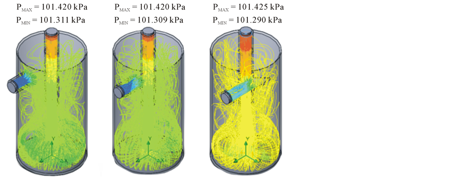 (d) (e) (f)
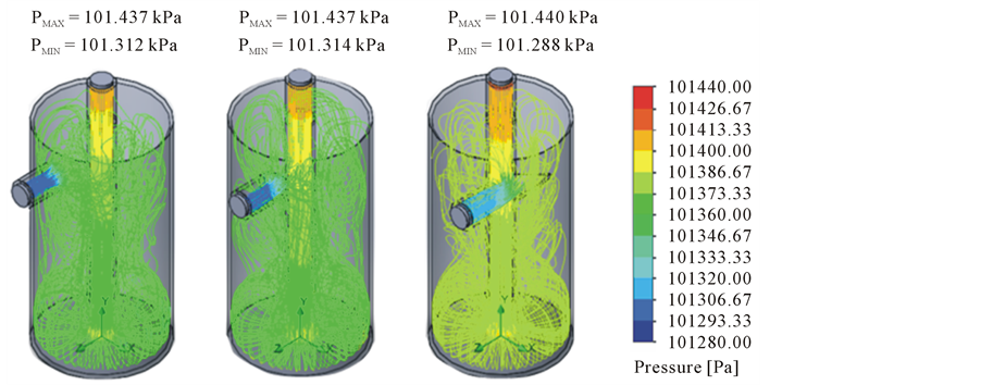 (g) (h) (i) (j)
Figure A1. Trajectory lines of particles of initial 9 chosen oil catch cans: (a) Xo = 30 mm, Yo = 0 mm; (b) Xo = 30 mm, Yo = 17.75 mm; (c) Xo = 30 mm, Yo = 35.5 mm; (d) Xo = 80 mm, Yo = 0 mm; (e) Xo = 80 mm, Yo = 17.75 mm; (f) Xo = 80 mm, Yo = 35.5 mm; (g) Xo = 130 mm, Yo = 0 mm; (h) Xo = 130 mm, Yo = 17.75 mm; (i) Xo = 130 mm, Yo = 35.5 mm; (j) Numerical contour scale.
Appendix II
 (a) (b) (c)
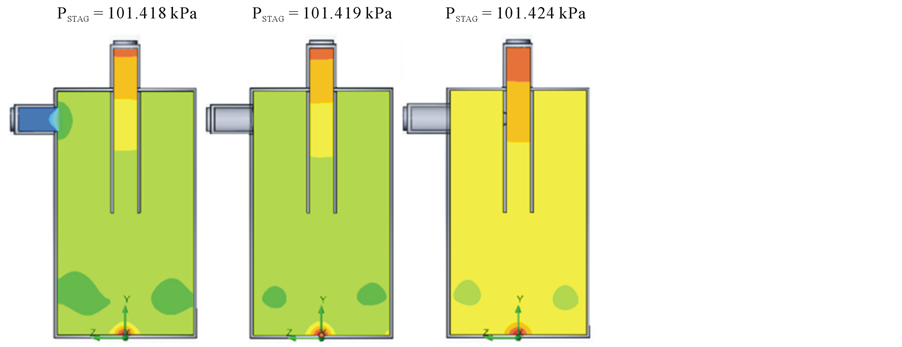 (d) (e) (f)
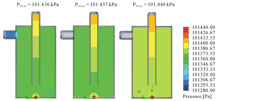 (g) (h) (i) (j)
Figure A2. Pressure contours of initial 9 chosen oil catch cans on YZ plane: (a) Xo = 30 mm, Yo = 0 mm; (b) Xo = 30 mm, Yo = 17.75 mm; (c) Xo = 30 mm, Yo = 35.5 mm; (d) Xo = 80 mm, Yo = 0 mm; (e) Xo = 80 mm, Yo = 17.75 mm; (f) Xo = 80 mm, Yo = 35.5 mm; (g) Xo = 130 mm, Yo = 0 mm; (h) Xo = 130 mm, Yo = 17.75 mm; (i) Xo = 130 mm, Yo = 35.5 mm; (j) Numerical contour scale.