Open Access Library Journal
Vol.02 No.04(2015), Article ID:68332,11 pages
10.4236/oalib.1101501
Iterative Method Based on the Truncated Technique for Backward Heat Conduction Problem with Variable Coefficient
Hongwu Zhang*, Xiaoju Zhang
School of Mathematics and Information Science, Beifang University of Nationalities, Yinchuan, China
Email: *zhhongwu@126.com
Copyright © 2015 by authors and OALib.
This work is licensed under the Creative Commons Attribution International License (CC BY).
http://creativecommons.org/licenses/by/4.0/


Received 1 April 2015; accepted 23 April 2015; published 27 April 2015
ABSTRACT
We consider a backward heat conduction problem (BHCP) with variable coefficient. This problem is severely ill-posed in the sense of Hadamard and the regularization techniques are required to stabilize numerical computations. We use an iterative method based on the truncated technique to treat it. Under an a-priori and an a-posteriori stopping rule for the iterative step number, the convergence estimates are established. Some numerical results show that this method is stable and feasible.
Keywords:
Ill-Posed Problem, Backward Heat Conduction Problem with Variable Coefficient, Iterative Method, Truncated Technique, Convergence Estimate
Subject Areas: Numerical Mathematics, Partial Differential Equation

1. Introduction
In this article, we consider the following backward heat conduction problem (BHCP) with variable coefficient
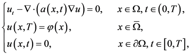 (1)
(1)
where  is a positive constant;
  denotes a bounded and connected open domain; the coefficient
  is assumed to be continuous and differentiable with respect to
 , respectively, and satisfying
 (2)
(2)
and
 (3)
(3)
our purpose is to determine  for
for  from the final measured data
  which satisfies
 ; here
  denotes the noisy level.
This problem is severely ill-posed and the regularization techniques are required to stabilize numerical computations [1] [2] . In past years, many authors have considered the regularization methods for the case  with constant coefficient
  (see [3] - [6] etc.). For the BHCP with variable coefficients, [7] investigated a case that the coefficient is independent of the time t, i.e.,
 . In 2010, Feng et al. [8] considered problem (1) and proved a condition stability result of Hölder type, then applied a truncated method to regularize it, and the corresponding convergence results have been given. On the other references for BHCP, we can see [9] - [12] , etc.
Followed the work in [8] , in this paper we use an iterative method to solve problem (1). The idea of this method (see Section 2) mainly comes from the reference [13] , where the authors investigated a backward heat conduction problem (BHCP) with densely defined self-adjoint and positive-definition operator. Recently this method has been used to solve some inverse problems of parabolic partial differential equation (PPDE). For instance, [14] investigated the same problem with [13] by rewriting the solution of inverse problem as the solution of a fixed point equation for an affine operator, and gave the convergence proof by using the functional analysis properties of the linear part of affine operator. Based on the variable relaxation factors, [15] treated the special case  with nonhomogeneous Dirichlet boundary condition and used the boundary element method (BEM) to implement numerical computation.
Inspired by [13] , in the present paper, we firstly adopt a similar method in [13] to obtain an iterative scheme, then truncate it to get our iterative method (see Section 2); here the data  for
for  will be determined. Under an a-priori and an a-posteriori stopping rule for the iterative step number, the convergence of the algorithm also will be given, and we can see that our convergence results are order optimal as
  in (1).
This paper is constructed as follows. In Section 2, we make a simple review for the ill-posedness of problem (1) and give the description of our iteration method. Section 3 is devoted to the convergence estimates under two stopping rules. Numerical results are shown in Section 4. Some conclusions are given in Section 5.
2. The Ill-Posedness and Description of the Iteration Method
2.1. The Simple Review of the Ill-Posedness for Problem (1)
We make a simple review for the ill-posedness of problem (1) (also see [8] ).
We denote  as the eigenvalues of negative Laplace operator
  defined in the space
 , and satisfy
 (4)
(4)
Further, we suppose that the corresponding eigenfunctions  satisfy
 (5)
(5)
then the eigenfunctions  form an orthonormal basis of
 .
.
From [8] , we know that the unique solution of problem (1) can be expressed as
 (6)
(6)
where  denotes the inner product in
 .
.
Setting , use the mean value theorem of integrals, for every fixed t, there exists some points
 , such that
 (7)
(7)
from (5) and the integration formula by parts, we know
 (8)
(8)
thus, the solution (6) can be rewritten as
 (9)
(9)
From (9), it can be observed that  tends to infinity as n tends to infinity, so in order
to recovery the stability of solution  given by (6), the coefficient
  must decay rapidly. However, such a decay usually cannot occur for the measured data
 , thus we have to use a regularization technique to restore numerical stability.
2.2. The Description of Iteration Method
In this subsection, we give our iteration method. Firstly, given  as an initial guessed value for
 , this method consist in solving the parabolic type equation
 (10)
(10)
this is a direct problem, use the similar method as in [8] , we can derive that the solution of problem (10) can be expressed as
 (11)
(11)
Now, for , let us choose a positive constant r, we need to solve the direct problem sequence of parabolic type equation
 (12)
(12)
then, for , we can obtain the solution of problem (12) is as follow
 (13)
(13)
Take , such that
 , and denote
 , then combine with (13), we can obtain the following iteration scheme
 (14)
(14)
Let the exact and noisy data  and satisfy
 (15)
(15)
where  denotes the
  -norm, the constant
  denotes a noise level. Then for the noisy data
 , the iteration scheme can be expressed by
 (16)
(16)
and we note that
 (17)
(17)
Now, we truncate (16) to obtain the following our iterative algorithm
 (18)
(18)
where N is a positive constant, which plays a role of the regularization parameter.
For simplicity, we take the initial guess as zero, then our iterative scheme becomes
 (19)
(19)
Further, we suppose that there exists a constant , such that the following a-priori bound holds
 (20)
(20)
3. Convergence Estimate
3.1. An A-Priori Stopping Rule
In the iterative process, the iterative step number k can be chosen by the a-priori and a-posteriori rules. In this subsection, we choose it by an a-priori rule and give the convergence estimate for the iterative algorithm.
Theorem 3.1. Suppose that u given by (6) is the exact solution of problem (1) with the exact data  and
and  is the iteration solution defined by (19) with the measured data
 . Let the measured data
  satisfy (15), and the a priori bound (20) is satisfied. If we choose the iteration step number
 , then for fixed
 , we have the following convergence estimate
 (21)
(21)
Proof. For , we define two functions
 , and
, and . Now we have the following two important inequalities [16] [17] .
 (22)
(22)
 (23)
(23)
where
 (24)
(24)
Use the triangle inequality, it is clear that
 (25)
(25)
From the Equations (6), (19) with the exact data , by the mean value theorem of integrals as in (7) of Subsection 2.1 and the integration by parts (8), and from the inequality (23), (24) with
 , a-priori bound (20), and
 , one can obtain that

On the other hand, from the Equation (19) with the exact and measured data ,
,  which satisfy (15), the inequality (22) with
 , the mean value theorem of integrals as in (7) and the integration by parts (8), we can get

From the above estimates of ,
,  , and the triangle inequality (25), we can obtain the convergence result (21).
3.2. An A-Posteriori Stopping Rule
In the iterative process, the a-priori stopping rule  needs the a-priori bound E for exact solution. And from the proof process of Theorem 3.1 we can notice that, for the iterative scheme (19), if an a-priori bound E is known, the bigger iterative step number k is, the better the iterative efficiency should be. However, a-priori bound generally can be not known, this is unfortunate for numerical computation. In order to make the convenient and accurate computation, instead of a-priori selection in Theorems 3.1, below we adopt the discrepancy principle [18] to control it, which is a kind of a-posteriori stop rule and the computation of iterative step number k does not need to know the a-priori bound of the exact solution.
For the iterative scheme (19), we control the iterative step number k by the following form
 (26)
(26)
where  is a constant,
  denotes the first iterative step which satisfies the first inequality of (26).
Theorem 3.2. Suppose that u given by (6) is the exact solution of problem (1) with the exact data  and
and  is the iteration solution defined by (19) with the measured data
  which satisfy (15). If the a priori bound (20) is satisfied and the iterative step
  is chosen by (26), then for fixed
 , we have the following convergence estimate
 (27)
(27)
Proof. Firstly, for the estimate of , adopting the similar procedure as in Theorem 3.1, from the inequality (22) with
 , (15), we have

Below, we estimate . From the scheme (19), the first inequality of stopping rule (26), and the orthogonal property of
 , it can be noted that
 (28)
(28)
then, we get
 (29)
(29)
Now, from the Equations (6), (19) with the exact data , by the mean value theorem of integrals as in (7) and the integration by parts (8), and from the inequalities (23), (24) with
 , (29), a-priori bound (20), one can derive that

From the above estimates of  and
and , the convergence result (27) can be obtained.
Remark 3.3.
For the a-priori case, in problem (1) and the inequality (2), if we take  and choose
 ,
,
then it can be obtained that

Note that,  , then it can be derived the following order optimal convergence result [19]
 (30)
(30)
where
 .
.
Similarly, for the a-posteriori case, we can derived the convergence result of order optimal
 (31)
(31)
where .
.
4. Numerical Implementations
In this section, we use a numerical example to verify how this method works. Since the ill-posedness for the case at  is stronger than the case of
 , here we are only interested in the reconstruction of the initial data
 .
.
Example. We take , and consider the following direct problem
 (32)
(32)
where ,
,  with the domain
 , its eigenvalue and the eigenfunction are
 ,
,  , respectively.
As in (10), (11), the solution of problem (32) can be written as
 (33)
(33)
here, . We choose the exact data as
 (34)
(34)
and the measured data  is given by
 , where
  is the error level.
In addition, we define the relative root mean square errors (RRMSE) between the exact and approximate solution is given by
 (35)
(35)
In order to make the convenient and accurate computation, we adopt the a-posteriori stopping rule (26) to choose the iterative step k. During the computation procedure, we take ,
,  to compute the iterative solution
  by (19) with
 .
.
For , the numerical results for
 ,
,  constructed from
  with
with  are shown in Figure 1. For
 , the numerical results for
 ,
,  constructed from
  are shown in Figure 2. For the constructed case from
 , the relative root mean square errors (RRMSE) and iterative number k with
  are shown in Table 1.
 (a) (b)
 (c) (d)
Figure 1. . (a)
. (a)  from
from ; (b)
; (b)  from
from ; (c)
; (c)  from
from ; (d)
; (d)  from
from .
.
 (a) (b)
 (c) (d)
Figure 2.  and
and  from
from . (a)
. (a) ; (b)
; (b) ; (c)
; (c) ; (d)
; (d) .
.

Table 1. The RRMSE generated from .
.
From Figure 1, Figure 2 and Table 1, we can see that our proposed method is stable and feasible. Figure 1 indicates that, with the increase of T, the construction effects become worse, this is because the information of final data will become less when T becomes big. From Figure 2 and Table 1, we note that the smaller the  is, the better the computed efficiency is. This is a normal phenomena in the backward heat conduction problem (BHCP).
5. Conclusion
An iterative method is based on the truncated technique to solve a BHCP with variable coefficients. Under an a- priori and an a-posteriori selection rule for the iterative step number, the convergence estimates are established. Some numerical results show that this method is stable and feasible.
Acknowledgements
The authors appreciate the careful work of the anonymous referee and the suggestions that helped to improve the paper. The work is supported by the the SRF (2014XYZ08), NFPBP (2014QZP02) of Beifang University of Nationalities, the SRP of Ningxia Higher School (NGY20140149) and SRP of State Ethnic Affairs Commission of China (14BFZ004).
Cite this paper
Hongwu Zhang,Xiaoju Zhang, (2015) Iterative Method Based on the Truncated Technique for Backward Heat Conduction Problem with Variable Coefficient. Open Access Library Journal,02,1-11. doi: 10.4236/oalib.1101501
References
- 1. Hanke, M., Engle, H.W. and Neubauer, A. (1996) Regularization of Inverse Problems, Volume 375 of Mathematics and Its Applications. Kluwer Academic Publishers Group, Dordrecht.
- 2. Kirsch, A. (1996) An Introduction to the Mathematical Theory of Inverse Problems, Volume 120 of Applied Mathematical Sciences. Springer-Verlag, New York.
- 3. Cheng, J. and Liu, J.J. (2008) A Quasi Tikhonov Regularization for a Two-Dimensional Backward Heat Problem by a Fundamental Solution. Inverse Problems, 24, Article ID: 065012.
http://dx.doi.org/10.1088/0266-5611/24/6/065012 - 4. Feng, X.L., Qian, Z. and Fu, C.L. (2008) Numerical Approximation of Solution of Nonhomogeneous Backward Heat Conduction Problem in Bounded Region. Mathematics and Computers in Simulation, 79, 177-188.
http://dx.doi.org/10.1016/j.matcom.2007.11.005 - 5. Liu, J.J. (2002) Numerical Solution of Forward and Backward Problem for 2-D Heat Conduction Equation. Journal of Computational and Applied Mathematics, 145, 459-482.
http://dx.doi.org/10.1016/S0377-0427(01)00595-7 - 6. Qian, Z., Fu, C.L. and Shi, R. (2007) A Modified Method for a Backward Heat Conduction Problem. Applied Mathematics and Computation, 185, 564-573.
http://dx.doi.org/10.1016/j.amc.2006.07.055 - 7. Shidfar, A., Damirchi, J. and Reihani, P. (2007) An Stable Numerical Algorithm for Identifying the Solution of an Inverse Problem. Applied Mathematics and Computation, 190, 231-236.
http://dx.doi.org/10.1016/j.amc.2007.01.022 - 8. Feng, X.L., Eld’en, L. and Fu, C.L. (2010) Stability and Regularization of a Backward Parabolic PDE with Variable Coefficients. Journal of Inverse and Ill-Posed Problems, 18, 217-243.
http://dx.doi.org/10.1016/j.jmaa.2004.08.001 - 9. Ames, K.A., Clark, G.W., Epperson, J.F. and Oppenheimer, S.F. (1998) A Comparison of Regularizations for an Ill-Posed Problem. Mathematics of Computation, 67, 1451-1472.
http://dx.doi.org/10.1090/S0025-5718-98-01014-X - 10. Clark, G.W. and Oppenheimer, S.F. (1994) Quasireversibility Methods for Non-Well-Posed Problems. Electronic Journal of Differential Equations, 8, 1-9.
- 11. Denche, M. and Bessila, K. (2005) A Modified Quasi-Boundary Value Method for Ill-Posed Problems. Journal of Mathematical Analysis and Applications, 301, 419-426.
http://dx.doi.org/10.1016/j.jmaa.2004.08.001 - 12. Marbán, J.M. and Palencia, C. (2003) A New Numerical Method for Backward Parabolic Problems in the Maximum-Norm Setting. SIAM Journal on Numerical Analysis, 40, 1405-1420.
- 13. Kozlov, V.A. and Maz’ya, V.G. (1989) On Iterative Procedures for Solving Ill-Posed Boundary Value Problems That Preserve Differential Equations. Algebra I Analiz, 1, 144-170.
- 14. Baumeister, J. and Leiteao, A. (2001) On Iterative Methods for Solving Ill-Posed Problems Modeled by Partial Differential Equations. Journal of Inverse and Ill-Posed Problems, 9, 13-30.
http://dx.doi.org/10.1515/jiip.2001.9.1.13 - 15. Jourhmane, M. and Mera, N.S. (2002) An Iterative Algorithm for the Backward Heat Conduction Problem Based on Variable Relaxation Factors. Inverse Problems in Engineering, 10, 293-308.
http://dx.doi.org/10.1080/10682760290004320 - 16. Louis, A.K. (1989) Inverse und schlecht gestellte Probleme. B.G. Teubner, Leipzig.
http://dx.doi.org/10.1007/978-3-322-84808-6 - 17. Vainikko, G.M. and Veretennikov, A.Y. (1986) Iteration Procedures in Ill-Posed Problems. Nauka, Moscow.
- 18. Morozov, V.A., Nashed, Z. and Aries, A.B. (1984) Methods for Solving Incorrectly Posed Problems. Springer, New York.
http://dx.doi.org/10.1007/978-1-4612-5280-1 - 19. Tautenhahn, U. (1998) Optimality for Ill-Posed Problems under General Source Conditions. Numerical Functional Analysis and Optimization, 19, 377-398.
http://dx.doi.org/10.1080/01630569808816834
NOTES

*Corresponding author.