International Journal of Geosciences, 2011, 2, 293-309
doi:10.4236/ijg.2011.23032 Published Online August 2011 (http://www.SciRP.org/journal/ijg)
Adapted Caussinus-Mestre Algorithm for Networks of
Temperature Series (ACMANT)
Peter Domonkos
Centre for Climate Change (C3), Geography Department, University Rovira i Virgili, Campus Terres de l’Ebre,
Tortosa, Spain
Received March 19, 2011; revised April 28, 2011; accepted June 1, 2011
Abstract
Any change in technical or environmental conditions of observations may result in bias from the precise
values of observed climatic variables. The common name of these biases is inhomogeneity (IH). IHs usually
appears in a form of sudden shift or gradual trends in the time series of any variable, and the timing of the
shift indicates the date of change in the conditions of observation. The seasonal cycle of radiation intensity
often causes marked seasonal cycle in the IHs of observed temperature time series, since a substantial portion
of them has direct or indirect connection to radiation changes in the micro-environment of the thermometer.
Therefore the magnitudes of temperature IHs tend to be larger in summer than in winter. A new homogenisa-
tion method (ACMANT) has recently been developed which treats in a special way the seasonal changes of
IH-sizes in temperature time series. The ACMANT is a further development of the Caussinus-Mestre method,
that is one of the most effective tool among the known homogenising methods. The ACMANT applies a
bivariate test for searching the timings of IHs, the two variables are the annual mean temperature and the
amplitude of seasonal temperature-cycle. The ACMANT contains several further innovations whose effi-
ciencies are tested with the benchmark of the COST ES0601 project. The paper describes the properties and
the operation of ACMANT and presents some verification results. The results show that the ACMANT has
outstandingly high performance. The ACMANT is a recommended method for homogenising networks of
monthly temperature time series that observed in mid- or high geographical latitudes, because the harmonic
seasonal cycle of IH-size is valid for these time series only.
Keywords: Statistical Method Development, Observed Climatic Data, Temperature, Time Series Analysis,
Data Quality Control, Homogenization, Efficiency
1. Introduction
For achieving reliable information about climate vari-
ability, large amount of observed time series of high
quality is needed. One principal tool for improving data
quality is the application of statistical homogenisation. In
the recent decades large number of homogenisation
methods have been developed and applied for homoge-
nising climatic time series. In these methods wide range
of statistical tools are applied for detecting change-points
or trends of non-climatic origination (i.e. inhomogenei-
ties [IH]) in observed meteorological time series. The
main tools of IH detection are 1) examination of accu-
mulated anomalies [1], 2) rank-order statistics [2,3], 3)
multiple linear regression [4,5], 4) t-test based examina-
tions [6,7], 5) multiple analysis with Fisher-test [8], 5)
fitting step-function [9]. Looking through reviewing arti-
cles about homogenisation methods [10-17] it can be
seen that we know many details about homogenisation
methods, but uncertainties still exist about their efficien-
cies, or with other words, about the practical usefulness
of individual methods.
The recently developed ACMANT homogenisation
method has some characteristics those are absolutely new,
and may influence positively the effectiveness of homo-
genisation. The most important innovation in ACMANT
is that it uses bi-variable test for detecting IHs in
monthly series of temperatures. The two variables are the
annual mean temperature and the amplitude of seasonal
cycle. Considering that the sizes of IHs in temperature
series often have seasonal cycle of considerable ampli-
tude [18,19], the selected two variables often have

P. DOMONKOS 294
change-points in the same time. The chance of right de-
tection increases when the change-points with common
time-points are searched with unified test for the two
variables. In ACMANT IHs with gradually changing
deviation from the correct values are approached by se-
ries of change-points, similarly as in many other ho-
mogenisation methods.
The paper describes the operation of the whole homo-
genisation procedure, discusses its general properties,
and gives information about its effectiveness. The orga-
nisation of the paper is as follow: The next section gives
a general picture about the main properties of ACMANT,
and describes the conditions of its practical application.
Section 3 describes the main functions of ACMANT in
detailed. In section 4 the operation of ACMANT is
summarised and its steps are presented in the true se-
quence. In section 5 some verification results are pre-
sented. Finally, in section 6, the properties of ACMANT
and the verification results are discussed, and conclu-
sions are drawn. The paper has an appendix with the ex-
planation of symbols applied.
2. Main Properties of ACMANT
1) A fully automated method.
2) The use of ACMANT is recommended for tem-
perature series from mid- and high-latitudes, since its
algorithm supposes quasi-harmonic annual cycle of con-
siderable amplitude in IH-sizes.
3) Relative homogenisation method, thus it can be
used for networks, and not for solely time series. Basi-
cally, the ACMANT applies the traditional comparison
of candidate series—reference series pairs. Reference
series are always built from minimum two component
series. A speciality of ACMANT that if the time series of
the network have observed values for different time pe-
riods, it may use different reference series for different
sections of the same candidate series and the selection of
reference series is automatic.
4) ACMANT incorporates the best detection and cor-
rection algorithms of known homogenisation methods,
i.e. the detection part is based on the PRODIGE [9]
method, while the final correction of time series is made
with ANOVA [9].
5) Main novelties of ACMANT relative to PRODIGE:
a) It applies the Caussinus—Mestre detection method
jointly to two variables, i.e. to annual means, and sum-
mer-winter differences; b) Fully automatic generation of
reference series, c) Pre-homogenisation for preparing
composites of reference series of better quality than in
the raw dataset, d) Separated way of detection for
long-term IHs and short-term IHs; e) After the calcula-
tion of correction-terms by ANOVA, those IHs that turn
out to be insignificant are deleted from the list of IHs,
and the ANOVA procedure is repeated with a reduced
list of IHs.
6) Two types of IH-detection are included in
ACMANT, i.e. the Main Detection is for long-term IHs
(generally with at least 3 years duration), while the Sec-
ondary Detection is for large-size but short-term IHs.
Both detection segments are developed from the Caussi-
nus-Mestre detection algorithm.
7) The lengths of raw time series in a network can be
different, and they may cover different time periods. Any
candidate time series or a section of candidate series is
subdued to homogenisation with ACMANT if at least
two partner time series exist in the network that cover the
period of the candidate series or its section and have at
least 0.5 autocorrelation with the candidate series.
8) Time series often contain large number of missing
values. If the ratio of missing values exceeds some preset
thresholds in some section(s) of the time series that sec-
tions are classified non-applicable sections, while the
section with acceptable ratio of available data is the ap-
plicable section. According to this, raw time series are
generally split into three sections, i.e. one applicable sec-
tion and two non-applicable sections before and after the
applicable section. If the ratio of missing values is ac-
ceptably low in the tails of the time series, there are no
non-applicable sections in the time series. The minimum
ratio of available data is 25% in the first k years and last
k years of the applicable section, for any k, k =
{1,2,···,15}, as well as the minimum ratio is 16.7% for
any 30-year subsection of the applicable section. A time
series must not contain more than one applicable section
(i.e. the applicable section cannot be separated into two
parts by a long pause of observation). The minimum
length of applicable section is 30 years.
9) The ACMANT has own segments for filling miss-
ing data and for substituting outlier values. For this pur-
pose spatial interpolation is applied. However, data of
non-applicable sections are not treated, and they do not
used at all during the homogenisation procedure.
10) Input data-field for ACMANT: Monthly tempera-
ture characteristics with monthly time resolution. The
lengths of time series may be different, but the data-
fields of each series are required to be converted into a
common format (which format includes the same number
of data for each temperature series) in a way that missing
values are filled with –999.9. After the preparation only
4 parameters have to be introduced before application: a)
Length of time series, b) First year of time series, c)
Number of time series in the network, d) Identifier of
network.
11) The result of homogenisation is a) Timings and
sizes of inhomogeneities (IHs) for each series. b) Tim-

P. DOMONKOS295
ings of outliers. c) Filled data-gaps caused by missing
values or outliers inside the series. d) Homogenised time
series. Sizes of IHs are characterised with two variables:
a) shift in annual means, b) shift in the amplitude of sea-
sonal cycle.
3. Main Functions of ACMANT
3.1. Basic Definitions
Before the description of the operation of ACMANT,
definitions of some basic statistical concepts are pre-
sented.
Time average of series X (denoted with upper stroke):
1
1n
i
i
x
n
 X (1)
Standard deviation of series X:


2
1
1n
i
i
x
n




X
X (2)
Time average of section [j1, j2] of series X:

2
1
21
1
1
j
i
ij
x
jj 


j1, j2
X (3)
Note that standard deviation for selected section of
time series is defined and denoted with the same logic as
section-average by Eqution (3).
Derivation of anomaly for station s, year j and month
m:
,, ,,,,
1
,
1s
n
s
jms jmsim
i
sm
ax x
n

 (4)
Missing values are represented with xs,i,m = 0, while n’
stands for the number of available observed values in xs,m
in Eqution (4). Note that due to missing values the sim-
ple time-average cannot be used in Equation (4).
ACMANT counts with anomalies during its whole
procedure, only in the last step the climatic means (the
second term in the right hand of Equation (4)) are added
back to the homogenised anomaly series.
Spatial correlation:

,
12
,, , ,
1
,,,
111
gsgs gs
gs gs
gs
nhxhx
gh shghsh
hhhnh
gsgs gs
r
aa aa
nnn


 
 


  





gs gsgs gs
g hn,hxs hn,hx
AA
hn




(5)
In Equation (5) g and s denote stations, h is the serial
number of month from the beginning of time series (here
time has one dimension only), hngs, hxgs and n’gs denote
the first month, the last months and total number of
months, for which observed data exist in both series,
respectively. Missing values of Ag and As are represented
with 0 in Equation (5).
3.2. Filling the Gaps of Time Series
This operation can be considered as one step of the
preparation of time series, because further segments of
ACMANT require continuous data series. However, on
the other hand, this operation is part of the ACMANT,
and it is performed automatically.
The interpolation for a missing value of month h in the
candidate series (Ag) relies on the same date values of
surrounding stations. All the time series of minimum 0.4
spatial correlation with the candidate series are used in
the interpolation, if they have observed value for month
h. The interpolated value is a weighted average of the
anomalies of the partner time series in h. For this inter-
polation, section-anomalies (a[h1,h2]) are calculated for the
symmetric window (h1,h2] around h. The number of ob-
served values used (n’) is usually 100 or 101, i.e. the
procedure search h1 and h2 for which h2 – h = h – h1, and
n’ε [100,101]. However, when the window is 2 × 10
years wide, i.e. h2 – h1 = 240 and n’ is still smaller than
100, n’ε [30,99] is accepted. In case of h2 – h1 = 240, and
n’ < 30, the window-width widens further, and it stops
when n’ε [100,101], or when h2 – h1 = 360. Equation (6)
shows the calculation of section-anomalies for series s.

2
1
, ,1,2
1
'
h
,
s
h shh h
ih
aa
n

si
a
(6)
Missing values of As are represented with zero in
Equation (6).
The interpolated value is the weighted average anom-
aly of N* surrounding series which is added to the pe-
riod-average of Ag. The weights are the squared spatial
correlations. When the sum of squared correlations is
lower than a fixed threshold (0.64), zero anomaly
ag,h[h1,h2] = 0 is presumed with a certain or entire weight,
according to Equations (7) and (8).

2
1
*2
,, ,1,2
1
11
'
h
N
,
g
hgs shh h
si
ara
pn



gi
h
a

, (7)
*2
,
1
max 0.64,
N
g
s
s
p





r


(8)
The gap-filling has to be accomplished before the
other steps in ACMANT. However, the first estimations
are not final, after some steps of pre-homogenisation the
interpolation is repeated in the same way as it is pre-
sented here, but with the use of data of higher quality.
There is one difference in the second round of the inter-

P. DOMONKOS 296

polation process, namely n’ < 100 (more exactly: n’ε
[30,99]) for window (h1,h2] is expected only when h2 – h1
= 360.
3.3. Constructing Relative Time Series
3.3.1. General Rules of Constructing Relative Time
Series in ACMANT
ACMANT makes relative homogenisation which relies
on the spatial comparison of time series. The way of this
comparison basically follows the traditional rules intro-
duced by [20], and applied later widely [21,23]. The
relative time series are the arithmetical differences of the
candidate series, and the so-called reference series (F)
(Equation 9).
 

12 12
g,q
g
j,jgj,j
TAF (9)
In Equation (9) a section is defined for which the rela-
tive time series is calculated. This section cannot stretch
out the ends of any reference-composites, or the ends of
the candidate series.
Reference series are built from the composition of
neighbouring series around the candidate series. The
weights of individual composites depend on the spatial
correlations between first difference (increment) series.
In studies about homogenisation methods one can find
different recommendations about the usefulness of first
difference series, and about the optimal number of refer-
ence-components. For ACMANT the use of first differ-
ence series was selected (Equation (10)) for evaluating
spatial correlations, because possible large IHs might
affect more seriously the spatial correlations of raw time
series (R’), than the spatial correlations of first difference
series (R).
,,1,
s
hsh s
aa a

 
h
for (10)

1, 121
s
hn 
Spatial correlations for ∆A are calculated according to
Equation (5) with the only difference from that, that at
this stage there are no missing values in the series, thus
instead of n’ the length of the period examined must be
applied. Denoting with bg,s,h the product of ∆ag,h and
∆as,h, the equation can be written in a simpler form
(Equation (11)).

,
,gs
r








g
sgsgsgs gsgs
gs gsgs gs
gshn ,hxghn ,hxshn ,hx
ghn,hxshn ,hx
BAA
AA (11)
For determining the number of reference-components
(S), minimum thresholds for acceptable spatial correla-
tions are introduced. In the present version of ACMANT
this threshold is relatively low, generally r ≥ 0.4, al-
though for at least two of the components it has to be at
least 0.5. The application of the relatively low threshold
values relies on the outcome of some experiments ac-
cording to the use of a large number of reference com-
ponents usually results in good verification results, even
if the spatial correlations of some components are rela-
tively low. Its explanation is that the increase of refer-
ence components tends to reduce the mean effect of IHs
and noise in the reference components.
The acceptable minimum of S is 2, in the reverse case
homogenisation cannot be fulfilled with ACMANT. Note
that one pre-selected time series is often excluded from
the reference composites, it is because during the pre-
homogenisation the candidate series for which the pre-
homogenised reference composites will be used must not
be taken into account in any form to avoid non-desired
effects of a multiplied use of the same information for
the same pieces of data in the homogenisation procedure.
For this reason it may occur that the number of reference
composites is not more than 1.
The composition of reference series for a predeter-
mined section [j1,j2] of series Ag is presented by Equation
(12).



2
,
1
S
gs
s
g
r
w

12
12
12
sj,j
gj,j j,j
A
F (12)
In Equation (12) w stands for the total weight of the
reference composites that have acceptable spatial corre-
lation with the candidate series, and available data in
section [j1,j2] as well (Equation (13)).

2
,
1
S
g
s
g
s
w


12
j,jr (13)
3.3.2. Application of Homogenisation-Adjustment for
Components of Relative Time Series
When relative time series are created, the candidate se-
ries are always raw or outlier-filtered time series and
homogenisation-adjustments have not been applied ear-
lier for them, while for reference-composites, homog-
enisation-adjustments are usually applied if adjustment
factors are available for them at the contemporary phase
of the procedure. Note that in the description of the algo-
rithm (Sect. 4), certain deviations from these rules will
be mentioned.
3.3.3. Constructing Different Relative Time Series for
Different Sections of the Candidate Series
For sections of the candidate series distinct reference
series are often built when the number of available series
with adequately high spatial correlation is larger for a
section, than for the entire series. In this way usually
more than one relative time series are produced for one
candidate series.
Considering that more than one relative time series

P. DOMONKOS297
1,1
can be constructed for one candidate series, we apply an
index (q) for denoting the individual reference series for
the same candidate series, while index g will be omitted
hereafter (since the candidate series is fixed in this ex-
amination). Generally Q reference series belong to one
candidate series, they starts at year y1,1, y2,1,…yQ,1, while
their last years are y1,2, y2,2,…yQ,2. Note that the minimum
length of reference series (yq,2 – yq,1 +1) is 30 years, and
as reference series never extend over the borders of their
candidate series, Y also marks the borders of relative
time series.
The determination of the set of reference series has
four main phases. In phase 1 three time series are deter-
mined, 1) the one with the highest w (Fopt) 2) the one
with the earliest yq,1 (y1,1) and iii) the one with the latest
yq,2. Note that Fopt may have the earliest yq,1 and/or the
latest yq,2, thus the final number of reference series
originated from this phase can be lower than 3.
In phase 2 potential reference series are examined
whose starting year (yq,1) is after y1,1, but earlier than yopt,1.
Obviously, when yopt,1 – y1,1 < 2 , this phase is omitted.
During this examination each possible yq,1 is examined,
proceeding step-by-step from y1,1+1 until yopt,1 – 1. Two
parameters (p1 and p2) are monitored during this exami-
nation (Equations (14) and (15)).
1,1qq
py y

 (14)
2
1
q
q
w
pw  (15)
A new reference series is selected when 1) p2 ≥ 1.3, or
2) p1 ≥ 5 and p2 ≥ 1.1, or 3) p1 ≥ 10 and p2 ≥ 1.03, or 4)
p1 = 30. Once a reference series is selected, the examina-
tions are continued recursively by examining the poten-
tial starting years between yq,1 and yopt,1. It follows from
the written rules that a new reference series is selected
with 30 years distance in the starting years at latest.
However, when the selection is based on condition 4) (p1
= 30), two special cases need more detailed description,:
i) It may occur that the available reference composites
for yq–1,1+30 are the same as for yq–1,1. In this case, al-
though there is no new reference series, the procedure
continues with the virtual yq,1 that equals with yq–1,1+30.
ii) Although w usually increases between y1,1 and yopt,1,
p2 of lower than 1 may occur for a 30-year subsection. In
this case, the maximal p2 is searched for between yq–1,1+1
and yq–1,1+30, and the corresponding reference series is
selected. Especially, it may occur (very rarely for ob-
served climatic time series) that even the maximal p2
does not satisfy the minimum conditions for creating
reference series, and a discrete subsection of [yq–1,1+30,
yopt,1] cannot be subdued to homogenisation, meanwhile
other sections before and after that subsection can be.
In phase 3 the symmetric procedure is applied for po-
tential reference series with ending years between yopt,2
and yq(latest),2 than in phase 2, proceeding backwards,
step-by-step from yq(latest),2 – 1 until yopt,2 + 1.
In phase 4 the selected reference series are ordered
according to w, and multiple selections of the same ref-
erence series are excluded.
3.3.4. Unified Relative Time Series
We introduce the concept of unified relative time series
(T+). It will be used for calculating temporary corrections
and filtering outliers in the section of pre-homogenisa-
tion. T+ is a combination of Tq series. The reasoning of
its introduction is empirical, i.e. adjustment factors that
are derived from different relative time series, often re-
sult in relatively large artificial biases in the low fre-
quency variability of the adjusted time series, even if the
individual estimations of change-point effects are rela-
tively good. The concept of the unified relative time se-
ries exploits the fact, that a relative time series can be
modified with an arbitrary constant without any effect on
the estimation of adjustment factors.
The set of relative time series is ordered according to
the decreasing values of w belonging to the relevant ref-
erence series, then the T series are examined one-by-one
following this order. The values of T+ for year j are de-
termined when the condition of Tq includes tq,j is satisfied
first. In the calculation of values for T+ the relevant val-
ues of Tq are usually adjusted with the mean difference
between T+ and Tq according to Equations (16)-(18).
When j lies before the section(s) for which T+ has values
determined from the previously examined T series,
Equation (16) is applied, while Equation (17) is applied
in the opposite case.

*
1
*
1
1
,,
1Yp

j
qji qi
iY
tt tt
p



 

(16)

*
2
*
2
,,
1
1Y

j
qji qi
iY p
tt tt
p


 
 (17)
where



*
11,1 2,11,1
*
21,22,2
min,, ,
max,, ,
q
q
Yyyy
Yyyy





1,2
(18)
Notes:
1. Month-indexes for t and t+ are omitted from Equa-
tions 16 and 17, first for simplicity, and secondly be-
cause often some annual characteristics are used in the
homogenisation procedure instead of monthly values
(see Sect. 3.4.1).
2. Value p is preset before the calculation of unified

P. DOMONKOS 298
time series. The value is relatively low (p = 5) in the be-
ginning of the homogenisation procedure, but with the
advance of the homogenisation it is higher (up to 30).
The philosophy of limiting p stems from the fact that
unadjusted change-points may affect the apparent dif-
ference of T+ and Tq, therefore sections that are relatively
close to the newly determined values are used only. For
the very same reason p is lower in the beginning of the
homogenisation procedure, and with the decreasing in-
fluence of unadjusted change-points p increases.
3. The p applied can be lower than its predefined value
when the number of available value-pairs of T+ and Tq is
lower than the predefined value of p. When the number
of applicable p is lower than 3, adjustment is not made,
i.e. in this case tj
+ = tq,j. It is always the case for q = 1.
4. It is seldom, but may occur that previously deter-
mined values of T+ exist on both sides of the newly de-
termined values. Introducing Y1
’ for the starting year of
the right section and Y2
’ for the ending year of the left
section, and substituting Y1
* and Y2 * in Equations (16)
and (17) with them, the estimations of the adjustment
factors included in the referred formulas are calculated
first and they are denoted with E1 and E2, respectively.
Then a linear transition between E2 and E1 provides the
adjustment factors for the values between Y2
’ and Y1 ’
(Equation (19)).
12
,2 1
12 12
jqj
Yj jY
tt EE
YY YY




 


 (19)
3.4. Detecting IHs with the Main Detection
3.4.1. Detection Process
In the Main Detection the timings and sizes of IHs are
searched with fitting step-functions to two variables,
namely to the annual means (TM) and summer-winter
differences (TD) in relative time series (Equations (20)
and (21)). In the following description the index q of
relative time series is omitted.
12
,
1
12
j
m
m
j
t
tm   (20)
,5,6,7,8 ,11 ,12,1,2
0.5 0.5
3.5
j
jjjj jjj
j
ttttt ttt
td  
(21)
In Equation (21) the second index represents calendar
month.
Solutions with common timings of steps are consid-
ered only, and the minimum sum of squared errors is
searched in a similar way as it is described by [24], [9],
etc. (Equations (22) and (23)).

1
12
'22
2
0
[ ,,...]01
min
k
Kk
j
K
ii
jj jkij
tmc td













 kk
TMTD (22)
00j

, (23)
1K
j
L
L denotes the length of the period examined, in years,
c0 is constant, while the number of change-points for the
selected period is K’. k characterises not only the serial
number of change-points, but the serial number of sec-
tions between adjacent change-points too (Equation
(24)).



kk1
kj1,j
TM TM (24)
c0 represents the estimated significance of changes of
TD in comparison to that of TM in relative time series.
In its estimation not only the mean sizes, but the sig-
nal/noise rate also had to be taken into account. In the
present application c0 = 2–0.5.
For selecting the most appropriate K’, the Caussinus –
Lyazrhi criterion [25] is applied (Equations (25) and (26)).
22 2
10
0
22 2
0
1
()()( )
ln 1
()()
K
kk
k
L
ii
i
jj c
tmc td
G








 


















kk
TMTMTD TD
TM TD
(25)

2'
ln
1
K
G
L
L (26)
The Main Detection differs in two points from the
classic Caussinus-Mestre detection method:
1) Step functions are fitted to two variables,
2) The minimum distance between two change-points
is 3 time-units:
13 kk
jj


 (27)

'0 Kkk 

3.4.2. Selection of Relative Time Series
Q different relative time series (T1, T2, ···,TQ) are derived
for one candidate series, and they are ordered according
to the sum of squared correlations of the refer-
ence-composites (w1 > w2 >… wQ). Each of them is used
in the Main Detection, but frequently some sections of
the relative time series are used only. The algorithm of
the relative time series selection is as follows:
1) First the T1 series is used with its whole length. In
this step section [y1,1,y1,2] of the candidate series is ho-
mogenised.
2) When the first q relative time series has already
been used, Tq+1 is applied for sections that a) lie within
[yq+1,1,yq+1,2] and b) have not been homogenised with the
first q relative time series.
3) When Tq+1 is applied, the tails of the sections ho-

P. DOMONKOS299

1


1

mogenised with the previous T series are often over-
lapped. It means that when ag,e1 belongs to a section that
has been homogenised previously, but ag,e1-1 has not, and
e1 > yq+1,1, a d1-year long section after e1 – 1 is subdued
again homogenisation. The usual length of this overlap is
9 years, but an overlapping section is not allowed to ex-
tend over a) IHs detected in previous steps, b) ends of
Tq+1 (i.e. yq+1,1 and yq+1,2). Let the first IH after e1 be de-
noted by k1 then the length of overlap is determined by
Equation (28).

1111,2
min9, 1,1
q
dkeye


(28)
For tails that lie in the other ends of the previously
homogenised sections (i.e. whose last point is e2), the
overlap (d2) is calculated with the same logic (Equation
(29)).

22221,
min9, ,1
q
dekey


(29)
In Equation (29) k2 stands for the first IH before e2.
3.5. Secondary Detection
In the Secondary Detection short-term IHs are searched
in relative time series adjusted according to the results of
the Main Detection. This operation is performed only
when the maximum of accumulated anomalies in ad-
justed relative time series exceeds some predefined
thresholds. Adjusted relative time series and the timing
of the maximum of accumulated anomalies are denoted
with T* and H*, respectively. T* is examined in its
monthly resolution, and the section that is selected
around H* is not allowed to be longer than 60 months.
This section has two sub-sections, namely the search
of the maximum of accumulated anomalies and the de-
tection of IHs around H*.
3.5.1. Search of the Maximum of Accumulated
Anomalies
5-month and 10-month moving averages are calculated
for the normalised anomalies of Tq*. All the relative time
series of the candidate series are used (q = 1,2,···,Q). In
Equations (30) and (31) the calculation of accumulated
anomalies is shown for 5-month and 10-month periods,
respectively.

**
2,
,*
2
1
MA 55()
hqh
qh
ih
t
b




q
q
T
T (30)

**
4,
,*
5
1
MA10 10 ()
hqh
qh
ih
t
b




q
q
T
T (31)
Note that in Equations (30) and (31) i is not allowed to
be lower than 1 or higher than the number of months (nm)
*
h ≤ nm – 4 have to be satisfied for Equations (30) and
(31), respectively.
After having the
in Tq, therefore the conditions of 3 ≤ h ≤ nm – 2 and 6 ≤
accumulated anomalies (MA5(b) and
M
3.2. Detection of IHs around the Maximum of
1) Selection of relative time series
nd for that operation
av
H
h1,h2] of 60 months
le
A10(b)) for each Tq*, their maximums are determined.
The maximums are calculated without sorting the accu-
mulated anomalies according to q, and in this way only
two maximal values are obtained, one for MA5 and an-
other for MA10. In the present version, Secondary De-
tection is made only when max(MA5(b)) ≥ 2.0 or
max(MA10(b)) ≥ 1.4. When exists a H* for which the
former relation is satisfied, the timing of the maximum
of 5-month anomalies is used, while the timing of the
maximum of 10-month anomalies is used when only the
latter relation is satisfied.
5.
Accumulated Anomalies
A window is edited around H* a
ailable data are needed in both sides of H*. Usually the
Tq* of the highest w is used for which at least 20 data are
available in each side of H*. When non of the Tq* series
meet with this condition (because H* is close to one end
of the candidate series), all the Tq* series are examined
again, with less strict conditions. In the second round the
expected minimum of available data (in each side of H*)
is 10, and in the third round (if that is necessary) the
minimum threshold is 2 only.
2) Edition of window around*
Usually a symmetric window [
ngth is edited around H*, but the window must not
overlap IHs detected in earlier steps or any end of the Tq
series, therefore it can be narrower than 60 months. Let
suppose that K1 change-points has been detected in the
earlier steps of the homogenisation procedure for section
[1,H*] of the series, then the borders of the window are
determined by Equations (32) and (33).


1
11, 1 K
*
max 29,hHH (32)


1
*
21
min30, ,
K
hHHn

 m (33)
3) Detection of IHs in windows
s is again the Caussi-
nu
stant sections are substituted with harmonic
fu
The base of the detection proces
s-Mestre method. However, in the Secondary Detec-
tion the constant sections of step-function are substituted
with harmonic functions of annual cycle for sections of
longer than 9 months, and some other modifications also
exist relative to the original Caussinus-Mestre method.
The list of differences from the original method is as
follows.
a) Con
nction of annual cycle for sections longer than nine

P. DOMONKOS 300
minimum distance between two change-points
is
are allowed to be de-
te
on (34) is ap-
pl
months;
b) The
3 time-units, i.e. 3 months in this case, but Equation
(26) is applicable here otherwise;
c) Maximum two change-points
cted in a window [h1,h2]. (K’ = 0, 1 or 2)
Describing more detailed point i), Equati
ied for fitting harmonic function of annual cycle.

1
2π2πmm

sin cos
12 12
1,
hkkAB
kk
uc c
hH H



 



, (34)
cA and cB are general constants in the procedure, because
se of β’ = 0 the function is constant and this fact
sh
.6. Calculation of Adjustment Factors
.6.1. ANOVA
f IHs of individual time series makes it
NT the ANOVA operates within an auto-
m
the ANOVA is applied separately for
tw
.6.2. Homogenisation-Adjustments during the
After IHs identified, adjustment-
used for cal-
cu
they characterise the relation between the phase of the
annual cycle and calendar month. Their values are set to
have the modus of the harmonic functions at the solstices
(cA = –0.1031, cB = –0.9947). Between two adjacent
change-points, αk’ and βk’ are also constants, and their
most proper values are searched with iteration. For find-
ing the best fitting model (K’, as well as the most appli-
cable timings of change-points), the function fitting of
Equation (34) must be applied for each subperiod of the
examined window, then the model with the lowest
Caussinus—Lyazrhi score is selected. This operation
contains large number of calculations, but by applying an
economic algorithm, the computation time is kept fairly
short.
In ca
ows that the step-function is a special case of the func-
tion family applied here.
3
3
The interaction o
necessary to calculate the precise adjustment-terms by an
equation system. In ACMANT the ANOVA method is
applied. In brief, the application of ANOVA to calculate
adjustment-terms for correcting IHs, is based on the di-
vision of observed time series to three components,
namely to climate effect, stations effect (IH) and noise.
In [9] it is proved that the optimal estimation of adjust-
ment-terms is provided when the noise term is set to be
zero in the equation system, thus the ANOVA provides
the optimal estimation of adjustment-terms. The referred
study also contains the detailed description of the appli-
cation of ANOVA in the homogenisation of climatic
time series.
In ACMA
atic procedure, therefore a special attention is needed
to treat cases when the equation system has no determi-
nistic solution. It could occur when all the time series of
a network (those that are comparable in the homogenisa-
tion procedure) have a change-point in the same time. In
that case the behaviour of sections before and after the
common change-point is independent. To avoid this case
the smallest IH is cancelled if all time series show IH at
the same time.
In ACMANT
o annual variables (i.e. for TM and TD), then the
monthly correction-terms are derived from them (see
Sect. 3.6.3). The ANOVA is applied after the Main De-
tection, then it is repeated after the Secondary Detection,
and if the number of IHs is reduced at the end of the
procedure relying on posterior tests, the application of
ANOVA is repeated again. However, ANOVA is not
applied during the pre-homogenisation, because it is not
a tool for making step-by-step improvements in the
dataset.
3
Pre-Homogenisation
having the timings of
terms for executing homogenisation can be deduced di-
rectly from relative time series. Although a part of the
detected biases can be caused by the impreciseness of
reference series, adjustment-terms are always applied
with its full content to the candidate series.
The unified relative time series (T+) are
lating temporary adjustments. Let suppose that for IH
k* Equations (35) and (36) show the shifts in TM and
TD.
**k




k1 k
TMTM
*
(35)
**k




k1k
TDTD
*
(36)
If the number of detected IHs is K, the c
fe
umulated ef-
ct of IHs on the candidate series in year i, i ≤ k* is
characterised by Equations (37) and (38).

K
 
TM TM 
*
i
kk

k1k (37)

*
K
i
kk




k1 k
TDTD (38)
.6.3. Derivation of Monthly Correction-Terms U de- 3
If IH k* has the timing H(k*) in monthly scale and
notes the adjustment-term, it can be given for any year i
and month m within the period [H(k*-1)+1,H(k*)] by
Equation (39). Corrections from β are distributed among
the calendar months in a way that the annual cycle is a
harmonic function with its extreme values in the solstices,
and the degree of changes in td satisfies Equation (21).
These conditions determine the monthly constants (cm) in
Equation (39).

P. DOMONKOS301
c
,
*
K
imkm k
kk
u




 (39)
3.7. Outlier-Filtering
Outlier filtering is applied two times in ACMANT,
namely for raw time series first, then after some steps of
the pre-homogenisation it is applied again. The applied
method is the same in both cases, only one little differ-
ence will be mentioned below.
Two operations are performed in this step.
1) Anomalies with higher than 4 standard deviations
are filtered according to Equation (40).

,, 4 sqh
t  
s,q s,q
TT

(40)
For each series s and month h always the Ts,q of the
highest w is selected which contains h. Note that in the
first outlier-filtering the mean of Ts,q is considered to be
0, because for differences of raw anomaly series the ex-
pected value is 0.
2) If in a 10-month long period, more than one outliers
of the same sign occur according to i), a confirmation is
needed, because the accumulation of seeming outliers
might be caused by large long-term variability. Therefore
in this case a second operation is accomplished, in which
potential outliers are examined with the statistical prop-
erties of the time-neighbourhood. Nineteen-month long
windows are used for this purpose. The potential outlier
is confirmed when the deviation from the win-
dow-average is larger than 3.5 standard deviation of the
values within the window, but is not considered to be
outlier in the reverse case (Equation (41)). For this op-
eration, again the relative time series of the highest w,
but with available data around h is selected.
 

,3.5 qh
t 
 

q h9,h9q h9,h9
TT


(41)
Note that when the number of available data is less
than 9 in one side of the window, this calculation is made
in a narrower window. In this case, if another Ts,q series
(of lower w) contains data for a full-size window, the
calculation is repeated with that data, and the results are
overwritten by that.
4. The Algorithm of ACMANT
Homogenisation Method
After the main functions of ACMANT have been de-
scribed, in this section the operation of the whole proce-
dure is presented.
In the homogenisation procedure raw time series are
converted several times (by interpolation, outlier-filtering,
pre-homogenisation), thus they go through several stages
before achieving their final form. During the procedure
some earlier stages are preserved, and reused. To make
distinctions among different stages of the same series
stage-codes are introduced. The code of raw time series
is 0, and if the series does not have sufficient spatial cor-
relations with other time series it might remain un-
changed during the homogenisation procedure of the
network. However, the gap-filling is done even for these
series, thus the code 0 indicates raw but continuous time
series. The meaning of the codes:
0 – raw
1 – outlier-filtered
2 – two times outlier-filtered
3 – pre-homogenised without outlier filtering
4 – pre-homogenised and outlier-filtered
4a – one time series is excluded during the
pre-homogenisation
5 – pre-homogenised and two times outlier filtered
5a – one time series is excluded during the pre-ho-
mogenisation
6 – homogenised
The algorithm of ACMANT
Part I: Preparation
1. Calculation of anomalies (Equation (4)).
2. Calculation of spatial correlations (Equation (5)).
3. Filling of data gaps in each time series (Sect. 3.2).
The results are the series of code 0.
4. Calculation of first difference series (Equation (10))
and their spatial correlations (Equation (11)).
5. Creation of relative time series from series-0 (Sects.
3.3.1 and 3.3.3).
6. Outlier-filtering for each time series (Sect. 3.7), the
results are series-1.
7. Spatial correlations are recalculated from series-1.
8. Interpolation for substituting outliers for each time
series (Sect. 3.2). When an outlier was detected in a se-
ries g in the same year and month at which interpolation
occurred in another series (s ≠ g) at step 3, its value is
re-interpolated at this step.
Part II: Pre-homogenisation
1) Calculation of first difference series and their spa-
tial correlations from series-1.
2) Creation of relative time series (Sects. 3.3.1, 3.3.3)
and unified relative time series (in Sect. 3.3.4 in Equa-
tions 16 and 17 p = 5). Type of candidate series: 1. Type
of reference components: 1.
3) Use of the Main Detection (Sect. 3.4) for ranking
time series according to the degree of inhomogeneous
character. Let the timings of IH (k) be denoted by jk, the
mean estimated bias of [jk+1,jk+1] by uk’, then an indica-
tor (z) of the degree of inhomogeneous character for sec-
tion [jk1+1,jk2] is calculated by Equation (42).

P. DOMONKOS 302


2
1
2
1
1.2
21 1
k
kk
kk
kk
jju
z
jj










(42)
Maximums of z values are searched examining each
possible k1 – k2 pair (0 ≤ k1 ≤ k2 ≤ K), then time series are
ordered according to their maximal z values. The actual
form of Equation 42 was chosen after some experiments
regarding the efficiency achievable. – In this step multi-
ple relative time series are used for determining the tim-
ings of IHs (as usual), but the T+ is used for calculating
indicator z.
Steps 4 - 7. compose a block that is accomplished for
each series in the order determined in step 3.
4) Calculation of relative time series. Type of candi-
date series: 1. Type of reference composites: 4a when the
composite has already bean pre-homogenised, 1 other-
wise.
5) Main Detection.
6) Calculation of relative time series and T+ with the
exclusion of one of the possible composites, p = 10.
Type of candidate series: 1. Type of reference compos-
ites: 4 when the composite has already been homoge-
nised, 1 otherwise.
7) Homogeneity-adjustments (Sects. 3.6.2 and 3.6.3).
a) Input: series-0, adjustment-terms: from T+ of step 3,
type of results series: 3; b) Input: series-1, adjust-
ment-terms: from T+ of step 3, type of results series: 4; c)
Input: series-1, adjustment-terms: from T+ of step 6, type
of results series: 4a.
8) Calculation of first difference series and their spa-
tial correlations from series-4.
9) Calculation of relative time series. This step pre-
pares the repetition of outlier-filtering, and for this rea-
son the candidate series are without previous out-
lier-filtering. Type of candidate series: 3. Type of refer-
ence composites: 4.
10) Outlier-filtering. The results are series-5.
11) Calculation of spatial correlations from series-5.
12) Recalculation of interpolated values using series-4.
The primer results are series-5. Then from the interpo-
lated values the homogenisation-adjustments are sub-
tracted, and with these values the outliers in series-0 are
substituted. The results are series-2.
13) Calculation of relative time series and T+ with the
exclusion of one of the possible composites, p = 30.
Type of candidate series: 2. Type of reference compos-
ites: 5.
14) Homogenisation-adjustments (Sects. 3.6.2 and
3.6.3). Input: series-2, adjustment-terms: from T+ of step
13, type of result series: 5a.
Part III: Homogenisation
Note: In this part unified relative time series are not
used.
1) Calculation of relative time series. Type of candi-
date series: 2. Type of reference composites: 5a.
2) Main Detection.
3) Exclusion of one IH, if there occurs a common
timing of IHs for all time series. Then the least signifi-
cant IH is selected, based on the calculations of indicator
z* around the timings of the common IH (k), Eqution
(43).



222
11 0
*kkkk zjj c



 (43)
In Equation (43) αk and βk are determined with Equa-
tions (35) and (36). The smallest z* indicates the least
significant IH, then that is excluded from the list of de-
tected IHs.
4) Refining timings of IHs in monthly time scale. In
the Main detection annual characteristics are used only,
so the timings of IHs cannot be assessed with monthly
preciseness from that. Here, the relative time series (T)
of step 1 are used in monthly resolution. – The first esti-
mation for the timing of IH k is taken from step 2, and it
is the December of the year (j) detected. Then two-phase
harmonic functions are fitted in a 48-month wide win-
dow centred at December of year j. This fitting is made
in the same way as for the Secondary Detection (Eqution
(34)), but here the number of change-points is fixed to be
1 within the window. Further limitation is that the timing
of the change-point is searched up to 12 months distance
from the centre of the window. – For the calculations of
this step always the Tq of the highest w is selected that
contains the 48-month window around jk.
5) Calculation of correction-terms with ANOVA. In-
put field: series-2 and timings of IHs from steps 2-4. This
step consists of three operations: a) ANOVA for correc-
tion-terms in annual means (TM) (Sect. 3.6.1); b)
ANOVA for correction-terms in summer-winter differ-
ences (TD) (Sect. 3.6.1); c) Calculation of monthly cor-
rection-terms (Sect. 3.6.3). – In ACMANT the input
variables are introduced to ANOVA in monthly resolu-
tion, as at this phase of the procedure the timings of IHs
are available with monthly preciseness. Problems do not
occur in calculating α, since the calendar months are
nearly evenly distributed between any two adjacent
change-points. By contrast, the summer-winter differ-
ence is a characteristic which has no values in monthly
time-scale. The problem is tackled by applying moving
weighted averages of monthly anomalies, providing
monthly values in this way for ANOVA calculations
(Equation (44)).
  

*5
,66
*5
0.5
H
j
mH
mHmH mH
HH
tdc acca



 

H
(44)

P. DOMONKOS303
1
k
Examining Equation (44) it can be seen that TD’
characterises the summer-winter difference, and it has
monthly values. Values for cm’ are set in harmony with
Equation (21), (c1’= –1/3.5, c2’= –0.5/3.5, etc.).
6) Application of homogenisation-adjustments on
relative time series of step 1. Each Tg,q (q = 1,2,···,Q) is
adjusted with the adjustment-factors determined by step
5 for series g. The results are T*.
Steps 7 and 8 compose a block whose steps are ful-
filled cyclically as long as inner indicators show the ne-
cessity of the continuation of the cycle.
7) Calculation of the maximums of accumulated and
normalised anomalies in adjusted relative time series.
(Sect. 3.5.1). If one of the maximums exceeds the
pre-defined thresholds, step 8 follows, otherwise the
procedure continues with step 9.
8) Secondary Detection (Sect. 3.5.2). Step 7 follows,
but before that the section of time series that has already
subdued to Secondary Detection, is excluded from fur-
ther examinations of accumulated anomalies.
9) Calculation of correction terms with ANOVA. The
only difference relative to step 5 is that here the list of
IHs is supplied with the result of the Secondary Detec-
tion.
10) Application of correction-terms on series-2. The
results are series-6.
Part IV. Final adjustments
Some IHs might turn out to be insignificant after the
ANOVA calculations. They are removed, and the
ANOVA is repeated with the rest of the IHs. These steps
are fulfilled cyclically as long as there is no insignificant
IH after the ANOVA calculations.
1) The significance of each IH (k) is controlled with
t-test. The size of IH is characterised by the sum of ab-
solute values of αk and c0βk where αk and βk are deter-
mined with Equations (35) and (36). The periods to
which the shift is assigned are presented by Equations
(45) and (46).
1kk
lHH

 (45)
21k
lH H

 (46)
The standard deviation for both periods is considered
to be the same as the standard deviation of the relative
time series in which k was detected. Let the sum of l1 and
l2 be denoted by l, then statistic p* can be given by
Equation (47).


012
2
*kk
clll
pl



 (47)
Note that p* differs from regular t-statistics of l-2
freedom because it includes β, while σ characterises the
standard deviation of α only. – In the present application,
thresholds for selecting significant IHs equal to the regu-
lar thresholds (depending on l) for the 0.05 significance
level. If at least 1 IH is excluded, step 2 follows, other-
wise step 4.
2) Calculation of correction terms with ANOVA. The
only difference relative to step 5 of Part III is, that here
the list of IHs is altered relative to the previous calcula-
tions.
3) Application of correction-terms on series-2. The
results are series-6. Step 1 follows.
4) Long-term means of monthly temperatures are
added to the homogenised anomalies (Equation (48)). a*
marks homogenised anomalies and V stands for ho-
mogenised temperature series.
*
,, ,,,,
1
,
1s
n
s
jms jmsim
i
sm
va x
n

 (48)
5. Verification
5.1. Test-Datasets
In the COST HOME action (COST ES0601) a bench-
mark dataset with known artificial IHs was built by a
group of experts, and was announced [26] for the clima-
tological community, for comparing the results of dif-
ferent homogenisation methods. This benchmark consists
of 40 networks of 100-year long series of simulated
monthly temperatures, 40 networks of simulated precipi-
tation data and some networks with real observed data.
For verification purpose only the simulated temperature
data are used in this study, since in datasets of real ob-
servations the properties of inhomogeneities are never
known perfectly, thus exact verification cannot be per-
formed for them.
Half of the simulated networks was generated with
white noise background (synthetic data), while in the
other half of the networks the background noise mimics
the low-frequency variability of time series better (sur-
rogated data). The benchmark contains networks of 15
time series (25%), networks of 9 time series (25%) and
networks of 5 time series (50%). The spatial correlations
are high (often higher than 0.8) what is typical for tem-
perature networks of the last 100-150 years observations
in Europe and the US. The frequency of IHs varies
widely, but most networks contain a few large IHs and a
lot of small IHs. See more details in [26].
In this study another test dataset is also used. It con-
sists of 100 surrogated and 100 synthetic networks of
monthly temperature data. This dataset (referred as
benchmark-2 hereafter) was created exactly in the same
way as the benchmark dataset, the only difference is that
in benchmark-2 all the networks contain 9 time series
(50%) or 15 time series (50%).

P. DOMONKOS 304
5.2. Evaluation of Efficiency
The root mean squared error (RMSE) caused by IHs or
imperfect homogenisation was calculated for some sta-
tistical characteristics of raw time series (WR) and for that
of homogenised time series (WH). Then the efficiencies
were calculated by Eqution (49).
R
H
R
WW
Eff W

 (49)
The verified characteristics are: 1) RMSE of monthly
biases, 2) RMSE of biases in annual means, and 3)
RMSE of slope-biases in the linear trend for the entire
period of time series.
5.3. Efficiency Results
In January of 2010 the first evaluation of efficiencies was
presented for the participants of COST event, and some
of the results have been published [27]. It was found that
the performance of ACMANT is one among the most
effective homogenisation methods. However, the author
has found problems with the reliability of climatic trend
estimation of that version (ACMANTv0), particularly
when the method was used for homogenising small net-
works (N = 5). After the causes of the bias have been
identified, some modifications were made in ACMANT.
The present version (ACMANTv1, February, 2011) that
is described in this study contains several modifications
relative to ACMANTv0. In the ACMANTv0 neither
ANOVA, nor unified relative time series were used for
calculating correction-terms, but those terms were calcu-
lated using the same relative time series as in which the
IHs were detected. The lack of harmonisation among
individual assessments may cause accumulated biases in
the estimation of long term trends. Another change is
that in ACMANTv1 the modus of the annual cycle coin-
cide with solstices, why in ACMANTv0 they were in
mid-January and mid-July. However, in the bench-
mark-homogenisation I still used the seasonal cycle of
the earlier version, because it provides the best results for
the benchmark.
The ACMANTv1 produces better results than the
ACMANTv0 not only in the trend estimation, but also in
the reconstructions of other statistical properties of time
series. For the 40 simulated networks of the benchmark
the efficiency of trend-slope estimation increased from
0.400 to 0.745, that of the annual mean temperatures
increased from 0.516 to 0.661, and that of the monthly
mean temperatures increased from 0.434 to 0.553.
As since February 2010 I know the true positions of
IHs in the benchmark, another test dataset, the bench-
mark-2 was used for the verification of ACMANTv1.
Surprisingly, the results for benchmark-2 are slightly
even better, than the results for the former benchmark
(Figure 1). When the values for Figure 1 were calcu-
lated, the small networks (N = 5) of the benchmark were
excluded, for using test-datasets of the same statistical
properties. It can be seen that 1) for relatively large net-
works even the ACMANTv0 performed quite well, 2)
the ACMANTv1 has always better efficiency than the
ACMANTv0, 3) the blind-test results are slightly even
better than the results achieved in the benchmark, 4) the
results are better when synthetic data are homogenised in
comparison with the homogenisation of surrogated net-
works, 5) the efficiency in reducing the monthly RMSE
is slightly poorer than the reduction of the annual RMSE.
The author cannot explain why the efficiency results
are better for the benchmark-2 than for the benchmark.
The opposite relation should be expected, since the
ACMANTv1 contains some semi-empirical parameters
which were assumed based on experiments with the
benchmark. Perhaps the 20 networks of the benchmark
that were used for Figure 1 frequently contain difficult
coincidences of IH and noise-terms by accident, in com-
parison with the mean properties of the much larger
benchmark-2. Anyhow, the achieved performance is out-
standingly high. The author does not know other ho-
mogenisation method with similar or better efficiency.
6. Discussion and Conclusions
The development of ACMANT relies on previous an-
alyses of efficiencies of homogenisation methods [28],
[29]. Notwithstanding, the application of homogenisation
methods on such a complete dataset as the benchmark of
the COST HOME offered and offers further opportuni-
ties to reveal the efficiency characteristics of methods.
This study restricts to discuss characteristics whose im-
pacts to the efficiency of ACMANT are unambiguous.
Seven favourable characteristics and three still existing
shortcomings are discussed:
1) IH-sizes of temperature series usually have seasonal
cycle. It is caused by the fact that most of the IHs have
relation to the change of radiation-sheltering or other
radiation effects, and these effects are larger in summer
than in winter. Thus, following the annual cycle of radia-
tion intensity, most of temperature IH sizes have
quasi-harmonic cycle. The benchmark of COST HOME
contains these seasonal changes of IHs rather realistically.
The ACMANT applies a bi-variable test for detect IHs,
one variable is the annual mean (TM), and the other is
the summer - winter difference (TD). This way of detec-
tion is very effective, because a) The two variables often
have change-points with the same timings, thus the sig-

P. DOMONKOS 305
nal/noise ratio is better in a unified tests; b) The use of
summer-winter difference is more effective, than the use
of seasonal or monthly means, because the signal/noise
ratio is relatively high for the summer - winter difference
(TD is calculated from the values of eight monthly
means, and the noise decreases with the increase of the
0
10
20
30
40
50
60
70
80
90
100
%
0
10
20
30
40
50
60
70
80
90
100
%
0
10
20
30
40
50
60
70
80
90
100
SUR SYN
%
ACMANTv0 ACMANTv1ACMANTv1-blind
Figure 1. Efficiency in reducing the RMSE of monthly biases caused by IHs or imperfect homogenisation. Results for
ACMANTv0, ACMANTv1-benchmark and ACMANTv1- benchmark-2 are presented by dotted, striped and filled fields,
respectively. Upper part: RMSE of monthly values; mid-part: RMSE of annual means, bottom: RMSE of trend-slopes.

P. DOMONKOS 306
number of averaged values); c) Distinct analyses of sea-
sonal and monthly series may result in set of detected
change-points with poor seasonal coherence. In that case,
after having the primer results, a harmonisation is neces-
sary to obtain a realistic description of IH properties.
Considering that that harmonisation needs further esti-
mations loaded with uncertainties, it might cause biases
in the result. In contrast, when TM and TD are examined,
such a harmonisation is unnecessary, because the sea-
sonal cycles of IHs can be derived directly from the de-
tection result.
2) One base of the development is the Caussinus -
Mestre detection method. Verification results show that
the Caussinus - Mestre detection method is one of the
best among the existing methods [29].
3) According to some tests fulfilled with the Caussinus
- Mestre detection method, its performance has turned
out to be better, when detection of IHs with shorter than
3 time units is not allowed. It is likely, because noise can
produce IH-shaped changes in the very short time-scale
more frequently than in longer time-scale. The
ACMANT applies this experience.
4) In ACMANT the ANOVA is applied for calculating
corrections which method provides the optimal estima-
tions of correction-terms.
5) The pre-homogenisation of reference components is
favourable when information specific for the connection
between the candidate series and its references is not
utilised in that step. The pre-homogenisation included in
ACMANT improves the certainty of the estimation of
number of IHs and that of the timings of IHs.
6) When the assessment of IH-positions are relatively
confident at least for large-size IHs, the applied method
for finding the timings of IHs in monthly time-scale
gives improvement. Note that according to some ex-
periments with the COST-benchmark, the application of
the same technique in an earlier phase of the procedure
for assessing timings with monthly preciseness did not
result in any improvement of efficiency.
7) The calculation of correction-terms with ANOVA
may show that some IHs which seemed to be significant
in the detection process, do not have significance in the
final results. With the exclusion of the insignificant IHs
(their percentage was approximately 10% when the
COST-benchmark was used) a better estimation of cor-
rection-terms can be provided basing on the significant
IHs only.
Three shortcomings still wait for the application of
further developments.
1) The aim of the Secondary Detection is to identify
short-term but large-size IHs. However, as it operates
after the Main Detection, a) the results of the Main De-
tection have errors due to unfiltered large-size, short-
term IHs, b) the results of the Secondary Detection are
affected by the errors of earlier steps.
2) The ACMANT is a purely statistical procedure,
now it is impossible to use metadata (documental infor-
mation of technical or environmental changes in the ob-
servation) information within ACMANT. However, the
author thinks that the potential usability of metadata is
limited when the spatial density and spatial correlations
of data is appropriate to perform statistical homogenisa-
tion, since metadata do usually not contain quantitative
information about the degree of local effects.
3) The present method is applicable for monthly tem-
peratures from mid- or high-latitudes, and is not applica-
ble for other climatic variables. The ACMANT contains
innovations whose application would likely be useful for
homogenising other variables than monthly temperatures,
therefore further developments of homogenisation me-
thods are needed.
A task for the future is, to apply efficiency-tests of
wider properties of time series and data networks than
which are provided by the COST-benchmark. The para-
meterisation of ACMANT has to be checked or modified
relying on further tests.
Summarising, the ACMANT is a new homogenisation
method which has been developed for homogenising
mid- and high-latitude temperature series of observing
networks. It has outstanding efficiency among statistical
homogenisation methods. Its use is particularly recom-
mended for homogenising networks comprising large
number of time series with sufficient spatial correlations,
since the ACMANT is a fully automatic method.
The executable file of ACMANTv1 together with its
user-guide is freely downloadable from
http://www.c3.urv.cat/members/pdomonkos.html.
7. Acknowledgements
The research was funded by the COST ES0601 project
and by the Centre for Climate Change (C3) of University
Rovira i Virgili. The author thanks Victor Venema for
providing access to dataset benchmark-2.
8. References
[1] T. A. Buishand, “Some Methods for Testing the Homo-
geneity of Rainfall Records,” Journal of Hydrology, Vol.
58, No. 1-2, 1982, pp. 11-27.
doi:10.1016/0022-1694(82)90066-X
[2] H. B. Mann and D. R. Whitney, “On a Test of Whether
One of Two Random Variables is Stochastically Larger
than the other,” The Annals of Mathematical Statistics,
Vol. 18, No. 1, 1947, pp. 50-60.
doi:10.1214/aoms/1177730491
[3] J. R. Lanzante, “Resistant, Robust and Non-Parametric

P. DOMONKOS307
Techniques for the Analysis of Climate Data: Theory and
Examples, Including Applications to Historical Ra-
diosonde Stationdata,” International Journal of Clima-
tology, Vol. 16, No. 11, 1996, pp. 1197-1226.
doi:10.1002/(SICI)1097-0088(199611)16:11<1197::AID-
JOC89>3.0.CO;2-L
[4] A. R. Solow, “Testing for Climate Change: An Applica-
tion of the Two-Phase Regression Model,” Journal of
Climate and Applied Meteorology, Vol. 26, No. 10, 1987,
pp. 1401-1405.
doi:10.1175/1520-0450(1987)026<1401:TFCCAA>2.0.C
O;2
[5] L. A. Vincent, “A Technique for the Identification of
Inhomogeneities in Canadian Temperature Series,”
Journal of Climate, Vol. 11, No. 5, 1998, pp. 1094-1104.
doi:10.1175/1520-0442(1998)011<1094:ATFTIO>2.0.C
O;2
[6] H. Alexandersson, “A Homogeneity Test Applied to Pre-
cipitation Data,” Journal of Climatology, Vol. 6, No. 6,
1986, pp. 661-675. doi:10.1002/joc.3370060607
[7] X. L. Wang, Q. H. Wen and Y. Wu, “Penalized Maximal
t Test for Detecting Undocumented Mean Change in
Climate Data Series,” Journal of Applied Meteorology
and Climatology, Vol. 46, No. 6, 2007, pp. 916-931.
doi:10.1175/JAM2504.1
[8] T. Szentimrey, “Multiple Analysis of Series for Homog-
enization (MASH),” Second Seminar for Homogenization
of Surface Climatological Data, WMO, Geneva, 1999, pp.
27-46.
[9] H. Caussinus and O. Mestre, “Detection and Correction
of Artificial Shifts in Climate Series,” Journal of Royal
Statistics Society Series C, Vol. 53, No. 3, 2004, pp.
405-425. doi:10.1111/j.1467-9876.2004.05155.x
[10] T. C. Peterson and 20 co-authors, “Homogeneity Ad-
justments of in Situ Atmospheric Climate Data: A Re-
view,” International Journal of Climatology, Vol. 18, No.
13, 1998, pp. 1493-1517.
doi:10.1002/(SICI)1097-0088(19981115)18:13<1493::AI
D-JOC329>3.0.CO;2-T
[11] E. Aguilar, I. Auer, M. Brunet, T. C. Peterson and J.
Wieringa, “WMO Guidelines on Climate Metadata and
Homogenization,” WMO, Geneva, 2003.
[12] J.-F. Ducré-Robitaille, L. A. Vincent and G. Boulet,
“Comparison of Techniques for Detection of Discontinui-
ties in Temperature Series,” International Journal of
Climatology, Vol. 23, No. 9, 2003, pp. 1087-1101.
doi:10.1002/joc.924
[13] I. Auer, et al., “A New Instrumental Precipitation Dataset
for the Greater Alpine Region for the Period 1800-2002,”
International Journal of Climatology, Vol. 25, No. 2,
2005, pp. 139-166. doi:10.1002/joc.1135
[14] M. J. Menne and C. N. Williams Jr., “Detection of Un-
documented Changepoints Using Multiple Test Statistics
and Composite Reference Series,” Journal of Climate,
Vol. 18, No. 20, 2005, pp. 4271-4286.
doi:10.1175/JCLI3524.1
[15] M. J. Menne and C. N. Williams Jr., “Homogenization of
Temperature Series via Pairwise Comparisons,” Journal
of Climate, Vol. 22, 2009, pp. 1700-1717.
[16] M. Brunet, M, O. Saladié, P. Jones, J. Sigró, E. Aguilar,
A. Moberg, D. Lister, A. Walther, D. Lopez and C. Al-
marza, “The Development of a New Dataset of Spanish
Daily Adjusted Temperature Series (SDATS)
(1850-2003),” International Journal of Climatology, Vol.
26, No. 13, 2006, pp. 1777-1802. doi:10.1002/joc.1338
[17] M. Brunet, O. Saladié, P. Jones, J. Sigró, E. Aguilar, A.
Moberg, D. Lister, A. Walther and C. Almarza, “A
Case-Study/Guidance on the Development of Long-Term
Daily Adjusted Temperature Datasets,” WC-DMP-66/
WMO-TD-1425, 2008.
[18] P. Domonkos, “Application of Objective Homogenization
Methods: Inhomogeneities in Time Series of Temperature
and Precipitation,” Időjárás, Vol. 110, 2006, pp. 63-87.
[19] M. Brunet, J. Asin, J. Sigró, M. Bañon, F. García, E.
Aguilar, J. E. Palenzuela, T. C. Peterson and P. Jones,
“The Minimization of the Screen Bias from Ancient
Western Mediterranean Air Temperature Records: An
Exploratory Statistical Analysis,” International Journal
of Climatology, Early View 2011,
[20] T. C. Peterson and D. R. Easterling, “Creation of Homo-
geneous Composite Climatological Reference Series,”
International Journal of Climatology, Vol. 14, No. 6,
1994, pp. 671-679. doi:10.1002/joc.3370140606
[21] H. Alexandersson, and A. Moberg, “Homogenization of
Swedish Temperature Data. Part I: Homogeneity Test for
Linear Trends,” International Journal of Climatology,
Vol. 17, No. 1, 1997, pp. 25-34.
doi:10.1002/(SICI)1097-0088(199701)17:1<25::AID-JO
C103>3.0.CO;2-J
[22] M. Begert, T. Schlegel and W. Krichhofer, “Homogene-
ous Temperature and Precipitation Series of Switzerland
from 1864 to 2000,” International Journal of Climatol-
ogy, Vol. 25, No. 1, 2005, pp. 65-80.
doi:10.1002/joc.1118
[23] A. T. DeGaetano, “Attributes of Several Methods for
Detecting Discontinuities in Mean Temperature Series,”
Journal of Climate, Vol. 19, No. 5, 2006, pp. 838-853.
doi:10.1175/JCLI3662.1
[24] D. M. Hawkins, “On the Choice of Segments in Piece-
wise Approximation,” IMA Journal of Applied Mathe-
matics, Vol. 9, No. 2, 1972, pp. 250-256.
doi:10.1093/imamat/9.2.250
[25] H. Caussinus and F. Lyazrhi, “Choosing a Linear Model
with a Random Number of Change-Points and Outliers,”
Ann. Inst. Statist. Math, Vol. 49, No. 4, 1997, pp.
761-775. doi:10.1023/A:1003230713770
[26] COST HOME home-page.
http://www.meteo.uni-bonn.de/venema/themes/homogeni
sation/
[27] V. Venema, O. Mestre and the COST HOME Team,
“Benchmark Database,” EGU General Assembly, Vienna,
Austria, 3-7 May, 2010.
[28] P. Domonkos, “Testing of Homogenisation Methods:
Purposes, Tools and Problems of Implementation,” Pro-
ceedings of the 5th Seminar and Quality Control in Cli-
matological, Hungarian, 25-27 October 2006.

P. DOMONKOS 308
[29] Databases, (Ed. M. Lakatos, T. Szentimrey, Z. Bihari and
S. Szalai), WCDMP-No. 71, 2008, pp. 126-145.
[30] P. Domonkos, “Efficiency Evaluation for Detecting In-
homogeneities by Objective Homogenisation Methods,”
Theoretical and Applied Climatology, Early View 2011.
doi:10.1007/s00704-011-0399-7

P. DOMONKOS309
Appendix: Explanation of Symbols and
Acronyms
The list below contains the explanation of symbols those
are used throughout the paper. Note that one can find
further explanations in the text about contemporary use
of variables, as well as about some constants and pa-
rameters whose role varies in the paper. Bold capital
letter marks vector or matrix variable.
A - anomaly
∆A - first difference (increment) of anomalies
A* - adjusted anomaly
B - normalised anomaly
F - reference series
g - index of candidate series
G - penalty term
h - serial number of month in a series
hn - first month of a series
hx - last month of a series
H - timing of change-point in months
H* - timing of selected change-point (in months)
j - year
k - serial number of change-point or that of section
in fitted function
K - total number of detected change-points for a
time series
K’ - number of detected change-points for a section
of a time series
l,L - length of series in a selected examination
m - calendar month
n - whole length of time series in years
n’ - number of observed values in time series
N - number of stations
nm - length of relative time series in months
p* - statistic of t-test
q - serial number of relative time series
Q - number of reference series for a specified candi-
date series
R - spatial correlation between first difference series
R’ - spatial correlation
s - station
S - number of components of reference series
T - relative time series
T+ - unified relative time series
T* - corrected relative time series
TM - annual mean
TD - summer-winter difference
U - correction-term
u’ - summarised impact / correction-term belongs to
some selected IHs
V - homogenised temperature
w - sum of the squared correlations of reference
components
WR - error-term for raw time series
WH - error-term for homogenised time series
X - raw time series
Y1 - first year of relative time series
Y2 - last year of relative time series
z, z* - indicator of significance of IHs
α - shift in annual means at an IH
β - shift in summer-winter differences at an IH
σ - standard deviation
ACMANT – Homogenisation method developed by the
author: Adapted Caussinus-Mestre Algorithm for ho-
mogenising Networks of Temperature series.
ACMANTv0 – The version of ACMANT that took part
in the blind test experiment of the COST HOME.
ACMANTv1 – The version of ACMANT that is de-
scribed in this paper.
ANOVA – Equation-system based calculation method of
correction-terms for homogenising time series.
COST HOME / COST ES0601 – International scientific
action on the development and testing of homogenisation
methods. It is sponsored by the European Union.
IH – Inhomogeneity: technical-born bias from the true
climate in the series of observed data.
MA – moving average
PRODIGE – Homogenisation method that was devel-
oped by Caussinus and Mestre (2004).
RMSE – Root mean squared error.
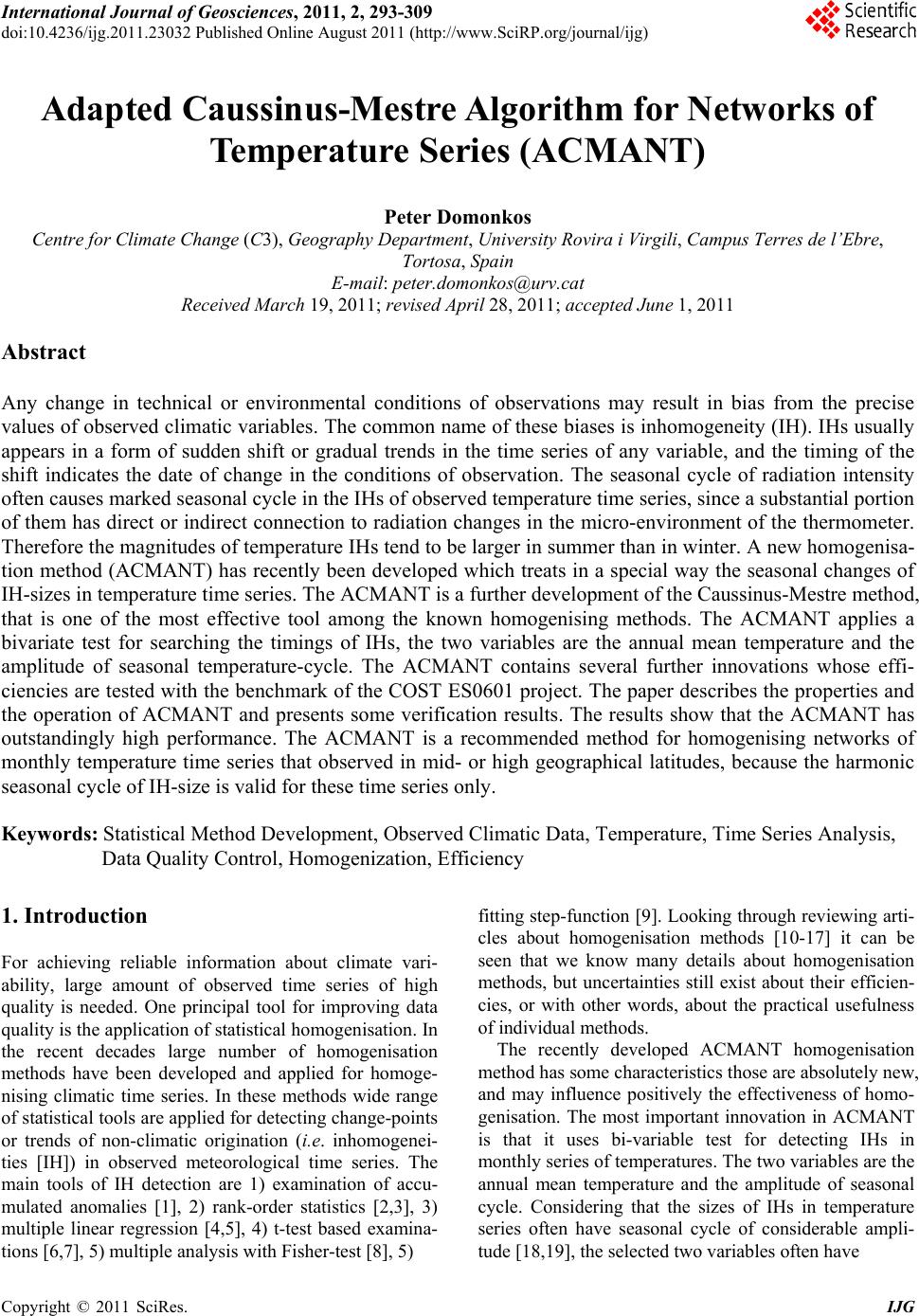