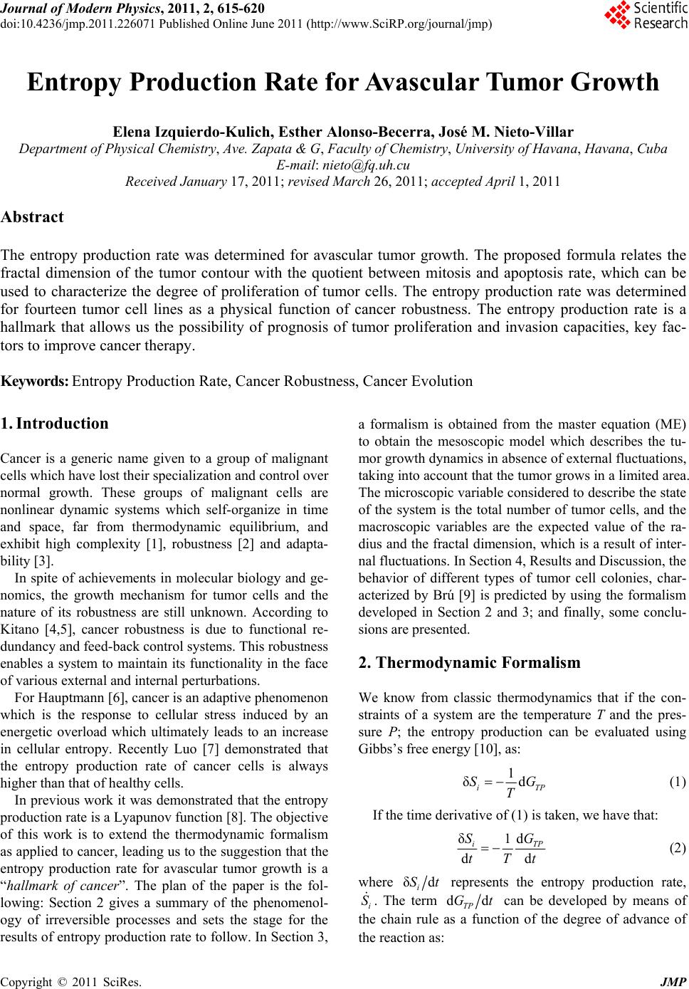Journal of Modern Physics, 2011, 2, 615-620
doi:10.4236/jmp.2011.226071 Published Online June 2011 (http://www.SciRP.org/journal/jmp)
Entropy Production Rate for Avascular Tu m or Growth
Elena Izquierdo-Kulich, Esther Alonso-Becerra, José M. Nieto-Villar
Department of Physi cal C hemistry , Ave. Zapata & G, Faculty of Chemistry, University of Havana, Havana, Cuba
Received January 17, 2011; revised March 26, 2011; accepted April 1, 2011
Abstract
The entropy production rate was determined for avascular tumor growth. The proposed formula relates the
fractal dimension of the tumor contour with the quotient between mitosis and apoptosis rate, which can be
used to characterize the degree of proliferation of tumor cells. The entropy production rate was determined
for fourteen tumor cell lines as a physical function of cancer robustness. The entropy production rate is a
hallmark that allows us the possibility of prognosis of tumor proliferation and invasion capacities, key fac-
tors to improve cancer therapy.
Keywords: Entropy Production Rate, Cancer Robustness, Cancer Evolution
1. Introduction
Cancer is a generic name given to a group of malignant
cells which have lost their specialization and control over
normal growth. These groups of malignant cells are
nonlinear dynamic systems which self-organize in time
and space, far from thermodynamic equilibrium, and
exhibit high complexity [1], robustness [2] and adapta-
bility [3].
In spite of achievements in molecular biology and ge-
nomics, the growth mechanism for tumor cells and the
nature of its robustness are still unknown. According to
Kitano [4,5], cancer robustness is due to functional re-
dundancy and feed-back control systems. This robustness
enables a system to maintain its functionality in the face
of various external and internal perturbations.
For Hauptmann [6], cancer is an adaptive phenomenon
which is the response to cellular stress induced by an
energetic overload which ultimately leads to an increase
in cellular entropy. Recently Luo [7] demonstrated that
the entropy production rate of cancer cells is always
higher than that of healthy cells.
In previous work it was demonstrated that the entropy
production rate is a Lyapunov function [8]. The objective
of this work is to extend the thermodynamic formalism
as applied to cancer, leading us to the suggestion that the
entropy production rate for avascular tumor growth is a
“hallmark of cancer”. The plan of the paper is the fol-
lowing: Section 2 gives a summary of the phenomenol-
ogy of irreversible processes and sets the stage for the
results of entropy production rate to follow. In Section 3,
a formalism is obtained from the master equation (ME)
to obtain the mesoscopic model which describes the tu-
mor growth dynamics in absence of external fluctuations,
taking into account that the tumor grows in a limited area.
The microscopic variable considered to describe the state
of the system is the total number of tumor cells, and the
macroscopic variables are the expected value of the ra-
dius and the fractal dimension, which is a result of inter-
nal fluctuations. In Section 4, Results and Discussion, the
behavior of different types of tumor cell colonies, char-
acterized by Brú [9] is predicted by using the formalism
developed in Section 2 and 3; and finally, some conclu-
sions are presented.
2. Thermodynamic Formalism
We know from classic thermodynamics that if the con-
straints of a system are the temperature T and the pres-
sure P; the entropy production can be evaluated using
Gibbs’s free energy [10], as:
1
δd
iTP
SG
T
 (1)
If the time derivative of (1) is taken, we have that:
δd 1
dd
iTP
SG
tTt
 (2)
where δd
i
St represents the entropy production rate,
i
S
. The term dd
TP
Gt can be developed by means of
the chain rule as a function of the degree of advance of
the reaction as:

E. IZQUIERDO-KULICH ET AL.
616
dd
dd
TP
TP
GG
tt


 


 (3)
where

TP
G

 —according to De Donder and Van
Rysselberghe [11]—represents the affinity A, with op-
posed sign, and the term ddt

is the reaction rate

.
Taking into account (2) and (3), we get:
δ1
d
ii
SSA
tT



(4)
The affinity can be calculated as [9]:

ln Ck
k
K
RT C


 


 (5)
where cfb
K
kk is the Guldberg-Waage constant
( and
f
b
kk are the forward and backward rate constants),
Ck is the concentration of the species k, whose
stoichiometric coefficients


k  are negative for reac-
tants and positive for a products. The formula (5) we
rewrite as:




ln
k
fkf
k
bkb
kC
RT kC




 


 (5a)
The reaction rate

 can be evaluated according to the
difference between the forward
f

and backward reac-
tion rates b

, as:


  
kk
fb fb kf kb
kC kC

  

 (6)
Substituting (6) and (5a) on (4) is obtained:

ln 0
f
ifb
b
SR

   


 (7)
The formula (7) is always positive by virtue of the
second law. As demonstrated as a proof in reference [8]
the relation (7) is a Lyapunov function, and thus provides
a directional criterion and stability for the dynamical
system, in other words, characterizes a complexity of the
system. As a matter of fact, we postulate the entropy
production given by (7) as a “hallmark of cancer” useful
to the prognosis of tumor proliferation.
3. Mesoscopic Model
To obtain a mathematical model to predict avascular
tumor growth, the following considerations were made:
First: The considered system is a tumor in vitro with a
circular geometry in 2D and an irregular contour, where
the increase of the number of cells n occurs because of
the reproduction of the contour cells. The total number of
cells n is the microscopic variable that describes the be-
havior of the system, and macroscopic variables consid-
ered were the tumor radius r and the fractal dimension of
the interface df , related by the expression:
2
π, r
n

(8)

1
2,
2
f
dGy (9)


1
ln
lim ,
ln
l
w
yl


 (10)
where 2
L




 is the area occupied by an individual cell,
w is an non-dimensional magnitude that express the
height difference between two points in the contour
separated by an non-dimensional distance l, and


Gy
is a linear function of y. Because the reproduction and
death of the cells on the contour are considered as sto-
chastic process, r is a stochastic variable who’s variance
is related with the contour roughness.
Geometrically, a tumor has the shape shown in Figure
1, in which the distance between the centre of the tumor
and the point at the interface more distant from the centre


H
L, the expected value of the tumor radius


RL,
and the difference between the maximum heights of two
points in the contour


WL are useful variables. (What
is the variable L?)
Second: As the contour rugosity is a property of the
tumour, not all the surface of radius H is covered by tu-
mour cells. If it is considered that internal fluctuations
scale with the area occupied by the microscopic entities
that characterize the tumour (tumour cells) then the per-
centage of the host area occupied by tumour cells de-
pends on the relation between the size of the entity and
the expected value of the area occupied by the tumour,
expressed by:
2
22
,
Rf
HR




(11)
H
R
W
Figure 1. Geometry representation of the tumour:


HLis
the distance betwee n the centre of the tumour and the point
at the interface most distant from the centre,


R
L is the
expected value of the tumour radius and


WL the dif-
ference between the maximum heights of two points on the
contour.

E. IZQUIERDO-KULICH ET AL.
617
where f is a function of the relation

2
R with the
following properties:
I think the function f is missing in these following 2
equations??
2
2
lim10; 1
f
o
R
Wd
R



 

 (12)
and
2
2
lim0; 2
f
R
Wd
R



 

 (13)
Third: Because the change of n depends of the prolif-
eration and death of the contour cells and if the formula
(7) is considered, then the transition probability per unit
of time Tr t–1 associated with the increases of n is writ-
ten a priori as:
0.5
r
Tn   (14)
While that the transition probability per unit of time
associated to the decrease of n, Td  t–1 is assumed as:
0.5
dd
Tkn (15)
where:

1;
;
da
kb F
bctc

 What is ctc?? (16)
2
2.
arn
FN
D
 (17)
In Equations (14) and (15)   t–1 is the cell reproduc-
tion rate constant, and kd  t–1 is the cell death rate con-
stant. The death rate constant kd includes a correction
term Fa, which represents the relation between the tu-
mour radius r and a characteristic length D of the area
(see Equations (16) and (17)) and takes into account the
finite area of the host. The term Fa is equivalent to the
relation between the total number of cells and the total
sites which can be occupied.
Considering the transition probabilities (14) and (15)
the master equation ME [12] which describes the prob-
ability behaviour P(n;t) of having n cells in time t is
written as:






1 0.5
1 0.5
0
;1;
11;,
;0 1,
n
n
Pnt nPnt
t
n
bnPnt
N
Pn






 



(18)
where a
n
 is the step operator.
Since the reproduction or death of a single cell pro-
duces a negligible effect on the system:
0,
n
n

 (19)
then the variable n can be considered continuous. If the
step operator is expressed in its differential form:
2
1
2
1
1,
2
nnn



 
 (20)
2
1
2
1
1,
2
nnn



 
 (21)
The Fokker-Planck equation (FPE) is obtained [12,13]
for P(n,t):



0.5 0.5
2
0.5 0.5
2
;1;
1
1;.
2
Pnt n
nb nPnt
tn N
n
nb nPnt
N n


 

 


 



 



  




(22)
If we take into account the following relations be-
tween the probability related to the microscopic P(n,t)
and the one related to the macroscopic variables P(r,t)
[13]:


;;;Pnt n Prt r

 (23)


;;
,
Pnt Prt
r
tnt




(24)
then the FPE related to the behavior of the macroscopic
variable is:
 

22
22 2
22
22
;11;
2
1
1;,
22
Prt rr
P
rt
tr Dr D
rPrt
r rD
 





 

  

 

 




  

















(25)
in which the relations among macroscopic and micro-
scopic rate constants are:
0.5
4




 (26)
0.5
.
4b




 (27)
In FPE (XXV), the first term on the right is a convec-
tive term related to the expected or deterministic value,
while the second term is a diffusive term related to the
fluctuations value. Taking into account that the macro-
scopically observed cell size  is independent of the
tumour size r2, we can consider that:
22
22 2
11
2
rr
DrD
 

 

 

 

 

 (28)

E. IZQUIERDO-KULICH ET AL.
618
in such a way that Equation (25) is written as:
 


2
2
22
22
00
;1;
1
1;,
22
;1
Prt rPrt
tr D
rPrt
r rD
Prt






 
 





















(29)
From the FPE (29) the expected radius of the tumour
R is obtained [12]:
22
22
0
dd
1; ,
dd
0
RRRR
tt DD
R
 

 




(30)
where  and  L. t–1 are the macroscopic parameters
associated to mitosis and apoptosis rate and

 L. t–1 is
the tumour growth rate (




) macroscopically
observed during the linear growth stage [9]; and for
variance
 :
2
22
0
d21,
d2
0
RR
tR
DD






 






(31)
The system of ordinary differential equations given by
(30) and (31) represents the mesoscopic model which
describes the tumour dynamics in absence of external
fluctuations considering the finite host area.
The stability analysis [14] shows that the radius grows
to a stable stationary state, also called dormant tumour
stage [15].
Forth: The tumour fractal dimension depends on the
physiological condition of active cells at the interface,
and it must include the reproduction and death rate con-
stants. To determine the characteristic fractal dimension
of the tumour, the right side of Equation (31) is equalled
to zero, so:
d0; ,
dDH t

 (32)
and the variance is expressed as:
22
22
1.
4
HR
RH







(33)
As the height difference between two points at the in-
terface is equivalent to the magnitude of internal fluctua-
tions, expressed by the square root of the variance [16],
the following non-dimensional expression is obtained
from Equation (33):
2
22
1,
4
l
wZ






(34)
where:
0.5
,w
H

 (35)
0.5
2,lR



 (36)
,
R
Z
H
 (37)


22
.
Z
fl (38)
In Equation (38) f(l2) is, according to the pre-estab-
lished considerations (see Equation (11)), a scale down
function which takes into account the fact that that inter-
nal fluctuations will depend on the size of the micro-
scopic entities and the size of the system.
Also, as there is a linear relation between the expected
value of the radius and the perimeter, the non-dimen-
sional variable l is equivalent to the distance between
two interface points. Consequently, the following scaling
relation can be assumed:




22 2
1- ,Zfl l (39)
So, Equation (34) is expressed as:
2
22
2.
4
l
wl






(40)
Substituting Equation (40) in (10) gives:


0.5
2
0.5
1
0.5
2
0.5
1
1
ln 2
4
lim ln
dln 2
4dln
limdd
,
l
l
ll
yl
lll
ll
yb



































 
















(41)
And finally (41) in Equation (9) gives:
12
1
2,
2
f
dC C
b





 






 (42)
where the constants C1 and C2 are evaluated taking into
account the interval of values physically possible that
can be obtained by the relation between the reproduction
and endogenous death rate constants. Then two extreme
cases appear: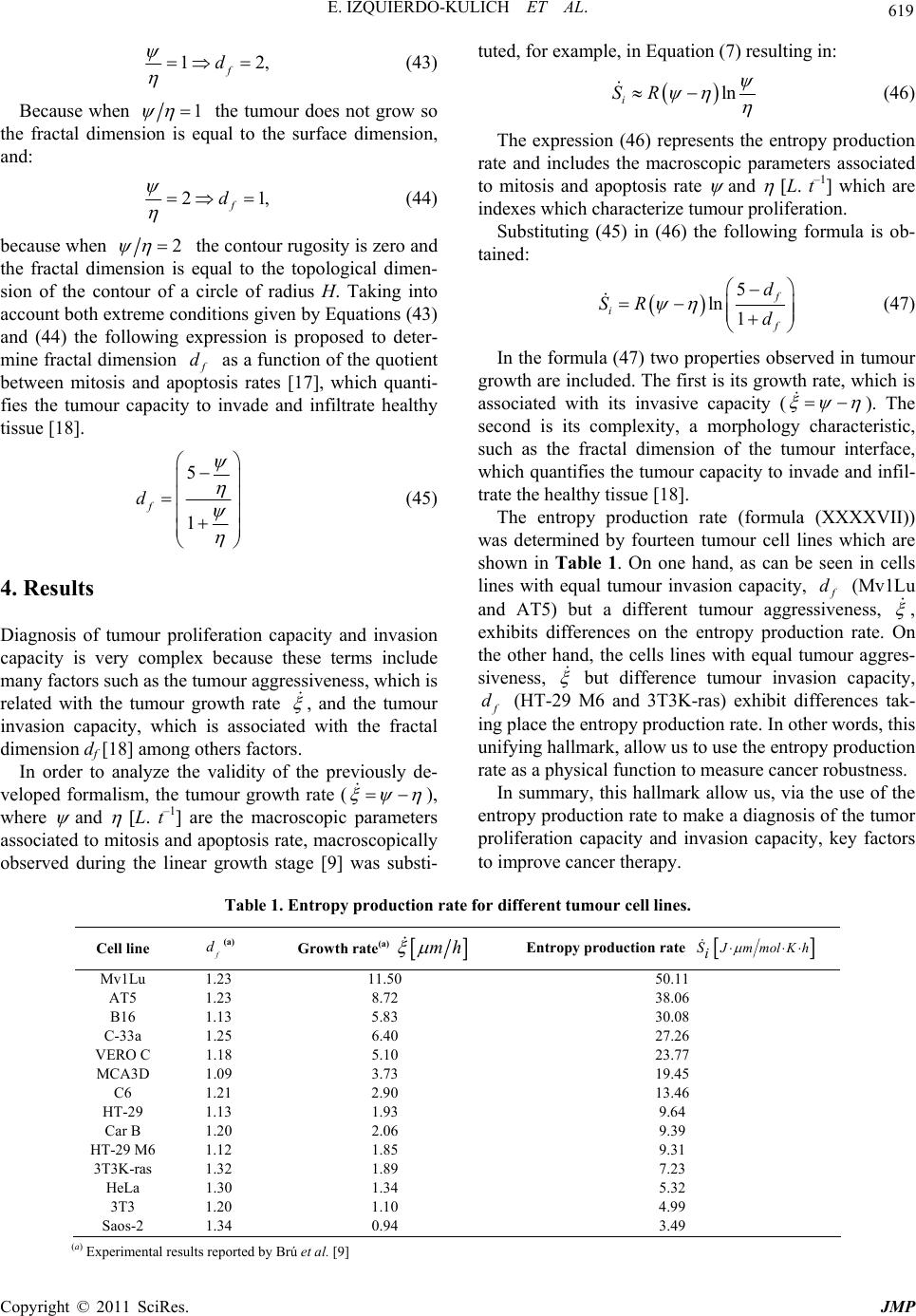

E. IZQUIERDO-KULICH ET AL.
619
12,
f
d


 (43)
Because when 1

  the tumour does not grow so
the fractal dimension is equal to the surface dimension,
and:
21,
f
d


  (44)
because when 2

  the contour rugosity is zero and
the fractal dimension is equal to the topological dimen-
sion of the contour of a circle of radius H. Taking into
account both extreme conditions given by Equations (43)
and (44) the following expression is proposed to deter-
mine fractal dimension
f
d as a function of the quotient
between mitosis and apoptosis rates [17], which quanti-
fies the tumour capacity to invade and infiltrate healthy
tissue [18].
5
1
f
d







 



(45)
4. Results
Diagnosis of tumour proliferation capacity and invasion
capacity is very complex because these terms include
many factors such as the tumour aggressiveness, which is
related with the tumour growth rate

, and the tumour
invasion capacity, which is associated with the fractal
dimension df [18] among others factors.
In order to analyze the validity of the previously de-
veloped formalism, the tumour growth rate (




),
where  and  L. t–1 are the macroscopic parameters
associated to mitosis and apoptosis rate, macroscopically
observed during the linear growth stage [9] was substi-
tuted, for example, in Equation (7) resulting in:

ln
i
SR




 (46)
The expression (46) represents the entropy production
rate and includes the macroscopic parameters associated
to mitosis and apoptosis rate  and  L. t–1 which are
indexes which characterize tumour proliferation.
Substituting (45) in (46) the following formula is ob-
tained:

5
ln 1
f
if
d
SR d 







 (47)
In the formula (47) two properties observed in tumour
growth are included. The first is its growth rate, which is
associated with its invasive capacity (

 
). The
second is its complexity, a morphology characteristic,
such as the fractal dimension of the tumour interface,
which quantifies the tumour capacity to invade and infil-
trate the healthy tissue [18].
The entropy production rate (formula (XXXXVII))
was determined by fourteen tumour cell lines which are
shown in Table 1. On one hand, as can be seen in cells
lines with equal tumour invasion capacity,
f
d (Mv1Lu
and AT5) but a different tumour aggressiveness,

,
exhibits differences on the entropy production rate. On
the other hand, the cells lines with equal tumour aggres-
siveness,

 but difference tumour invasion capacity,
f
d (HT-29 M6 and 3T3K-ras) exhibit differences tak-
ing place the entropy production rate. In other words, this
unifying hallmark, allow us to use the entropy production
rate as a physical function to measure cancer robustness.
In summary, this hallmark allow us, via the use of the
entropy production rate to make a diagnosis of the tumor
proliferation capacity and invasion capacity, key factors
to improve cancer therapy.
Table 1. Entropy production rate for different tumour cell lines.
Cell line f
d(a) Growth rate(a)


mh 
 Entr opy prod uction rate


J
mmolKhSi  

Mv1Lu 1.23 11.50 50.11
AT5 1.23 8.72 38.06
B16 1.13 5.83 30.08
C-33a 1.25 6.40 27.26
VERO C 1.18 5.10 23.77
MCA3D 1.09 3.73 19.45
C6 1.21 2.90 13.46
HT-29 1.13 1.93 9.64
Car B 1.20 2.06 9.39
HT-29 M6 1.12 1.85 9.31
3T3K-ras 1.32 1.89 7.23
HeLa 1.30 1.34 5.32
3T3 1.20 1.10 4.99
Saos-2 1.34 0.94 3.49
(a) Experimental results reported by Brú et al. [9]

E. IZQUIERDO-KULICH ET AL.
620
5. Acknowledgements
This work was support by a grant of the Higher Educa-
tion Ministry of Cuba.
6. References
[1] T. S. Deisboeck, M. E. Berens, A. R. Kansal, S. Torquato,
A. O. Stemmer-Rachamimov and E. A. Chiocca, “Pattern
of Self-Organization in Tumour Systems: Complex
Growth Dynamics in a Novel Brain Tumour Spheroid
Model,” Cell Proliferation, Vol. 34, 2001, pp. 115-134.
doi:10.1046/j.1365-2184.2001.00202.x
[2] H. Kitano, “Towards a Theory of Biological Robustness,”
Molecular Systems Biology, Vol. 3, 2007, p. 137.
doi:10.1038/msb4100179
[3] D. Rockmore, “Cancer Complex Nature,” Santa Fe Insti-
tute Bulletin, Vol. 20, 2005, pp. 18-21.
[4] H. Kitano, “Cancer Robustness: Tumour Tactics,” Nature,
Vol. 426, 2003, p. 125. doi:10.1038/426125a
[5] H. Kitano, “Cancer as a Robust System: Implications for
Anticancer Therapy,” Nature Reviews Cancer, Vol. 4,
2004, pp. 227-235. doi:10.1038/nrc1300
[6] S. Hauptmann, “A Thermodynamic Interpretation of Ma-
lignancy: Do Genes Come Later?” Medical Hypotheses,
Vol. 58, 2002, pp. 144-147. doi:10.1054/mehy.2001.1477
[7] L. F. Luo, “Entropy Production in a Cell and Reversal of
Entropy Flow as an Anticancer Therapy,” Frontiers of
Physics in China, Vol. 4, 2009, pp. 122-136.
doi:10.1007/s11467-009-0007-9
[8] J. M. Nieto-Villar, R. Quintana and J. Rieumont, “En-
tropy Production Rate as a Lyapunov Function in
Chemical Systems: Proof,” Physica Scripta, Vol. 68,
2003, pp. 163-165.
doi:10.1238/Physica.Regular.068a00163
[9] A. Brú, S. Albertos, J. L. Subiza, J. L. García-Asenjo and
I. Brú, “The Universal Dynamics of Tumour Growth,”
Biophysical Journal, Vol. 85, 2003, pp. 2948-2961.
doi:10.1016/S0006-3495(03)74715-8
[10] I. Prigogine, “Introduction to Thermodynamics of Irre-
versible Processes,” Wiley, New York, 1961.
[11] Th. De Donder and P. Van Rysselberghe, “Thermody-
namic Theory of Affinity, H. Milford,” Oxford Univer-
sity Press, London, 1936.
[12] N. G. Van Kampen, “Stochastic Processes in Physics and
Chemistry,” 3rd Edition, Elsevier, Amsterdam, 2007.
[13] C. W. Gardiner, “Handbook of Stochastic Methods: For
Physics, Chemistry and the Natural Sciences,” 3rd Edi-
tion, Springer-Verlag, Heidelberg, 2004.
[14] V. Anishchenko, V. Astakhov, A. Neiman, T. Vadisova
and L. Schimansky-Geir, “Nonlinear Dynamics of Cha-
otic and Stochastic Systems: Tutorial and Modern De-
velopments,” 2nd Edition, Springerr-Verlag, Heidelberg,
2007.
[15] V. A. Kuznetsov, I. A. Makalkin, M. A. Taylor and A. S.
Perelson, “Nonlinear Dynamics of Immunogenic Tumours:
Parameter Estimation and Global Bifurcation Analysis,”
Bulletin of Mathematical Biology, Vol. 56, 1994, pp. 295-
231.
[16] A. L. Barabasi and H. E. Stanley, “Fractal Concepts in
Surface Growh,” Cambridge University Press, Cambridge,
1995. doi:10.1017/CBO9780511599798
[17] E. Izquierdo and J. M. Nieto-Villar, “Morphogenesis of
the Tumour Patterns,” Mathematical Biosciences and
Engineering, Vol. 5, 2008, pp. 299-313.
[18] L. Norton, “Conceptual and Practical Implications of
Breast Tissue Geometry: Toward a More Effective, Less
Toxic Therapy,” Oncologist, Vol. 10, 2005, pp. 370-381.
doi:10.1634/theoncologist.10-6-370