Wireless Engineering and Technology
Vol.2 No.1(2011), Article ID:3793,7 pages DOI:10.4236/wet.2011.21005
An Efficient Method to Reduce the NumericalDispersion in the HIE-FDTD Scheme
![]()
School of Electronic and Information Engineering, Xi’an Jiaotong University, Xi’an, China.
Email: chenjuan0306@yahoo.com.cn
Received September 2nd, 2010; revised November 2nd, 2010; accepted November 18th, 2010.
Keywords: HIE-FDTD, Numerical Dispersion, Weakly Conditionally Stability
ABSTRACT
A parameter optimized approach for reducing the numerical dispersion of the 3-D hybrid implicit-explicit finite-difference time-domain (HIE-FDTD) is presented in this letter. By adding a parameter into the HIE-FDTD formulas, the error of the numerical phase velocity can be controlled, causing the numerical dispersion to decrease significantly. The numerical stability and dispersion relation are presented analytically, and numerical experiments are given to substantiate the proposed method.
1. Introduction
The finite-difference time-domain (FDTD) method [1] has been proven to be an effective means that provides accurate predictions of field behaviors for varieties of electromagnetic interaction problems. However, as it is based on an explicit finite-difference algorithm, the Courant–Friedrich–Levy (CFL) condition [2] must be satisfied when this method is used. Therefore, a maximum time-step size is limited by minimum cell size in a computational domain, which makes this method inefficiency for the problems where fine scale dimensions are used.
To relax the Courant limit on the time step size of the FDTD method, a three–dimensional (3-D) hybrid implicit-explicit finite-difference time-domain (HIE-FDTD) method has been developed recently [3]. In this method, the CFL condition is not removed totally, but being weaker than that of the conventional FDTD method. The time step in this scheme is only determined by two space discretizations, which is extremely useful for problems where a very fine mesh is needed in one direction. However, the numerical dispersion error of the HIE-FDTD scheme is larger than that of the conventional FDTD method.
In this letter, a simple and efficient approach for reducing the numerical dispersion of the 3-D HIE-FDTD method is proposed. Numerical results indicate that the numerical dispersion of the method can be notably reduced when a proper parameter is introduced [4]. As a result, the usefulness and effectiveness of the HIE-FDTD method can be significantly enhanced. The numerical dispersion of the new algorithm is studied analytically and validated by a numerical simulation, and the results are compared with both the standard HIE-FDTD method and the conventional FDTD method.
2. Formulations
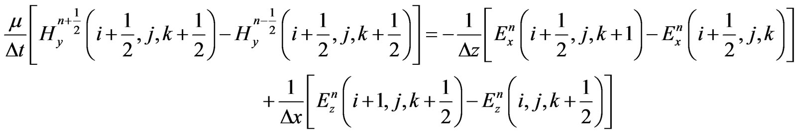
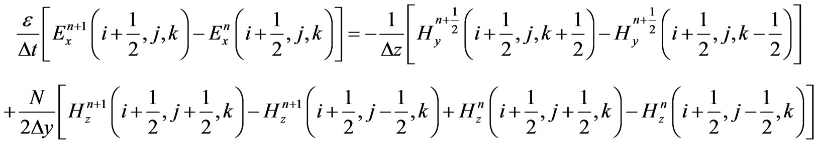
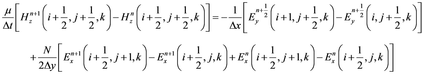
To reduce the numerical dispersion of the 3-D HIEFDTD method, parameter N is introduced into the HIE-FDTD discretization. The modified algorithm is described as follows:
 (1)
(1)
 (2)
(2)
 (3)
(3)
 (4)
(4)
 (5)
(5)
 (6)
(6)
 and
and  are the index and size of time-step,
  ,
,  and
and  are the spatial increments respectively in
 ,
,  and
and  directions,
  ,
, , and
, and  denote the indices of spatial increments respectively in
 ,
,  , and
, and  directions,
  and
and  are the permittivity and permeability of the surrounding media, respectively. When the value of parameter N is equal to 1, Equations (1)-(6) is the formulations of standard HIE-FDTD method [3].
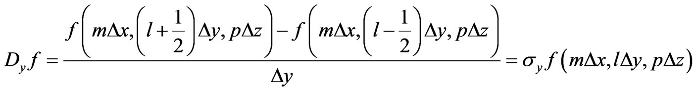
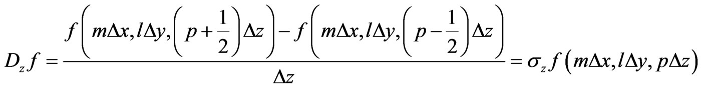
Obviously, updating of  component, as shown in Equation (3), needs the unknown
  component at the same time, thus the
  component has to be updated implicitly. Substituting Equation (5) into Equation (3), the equation for
 field is given as:
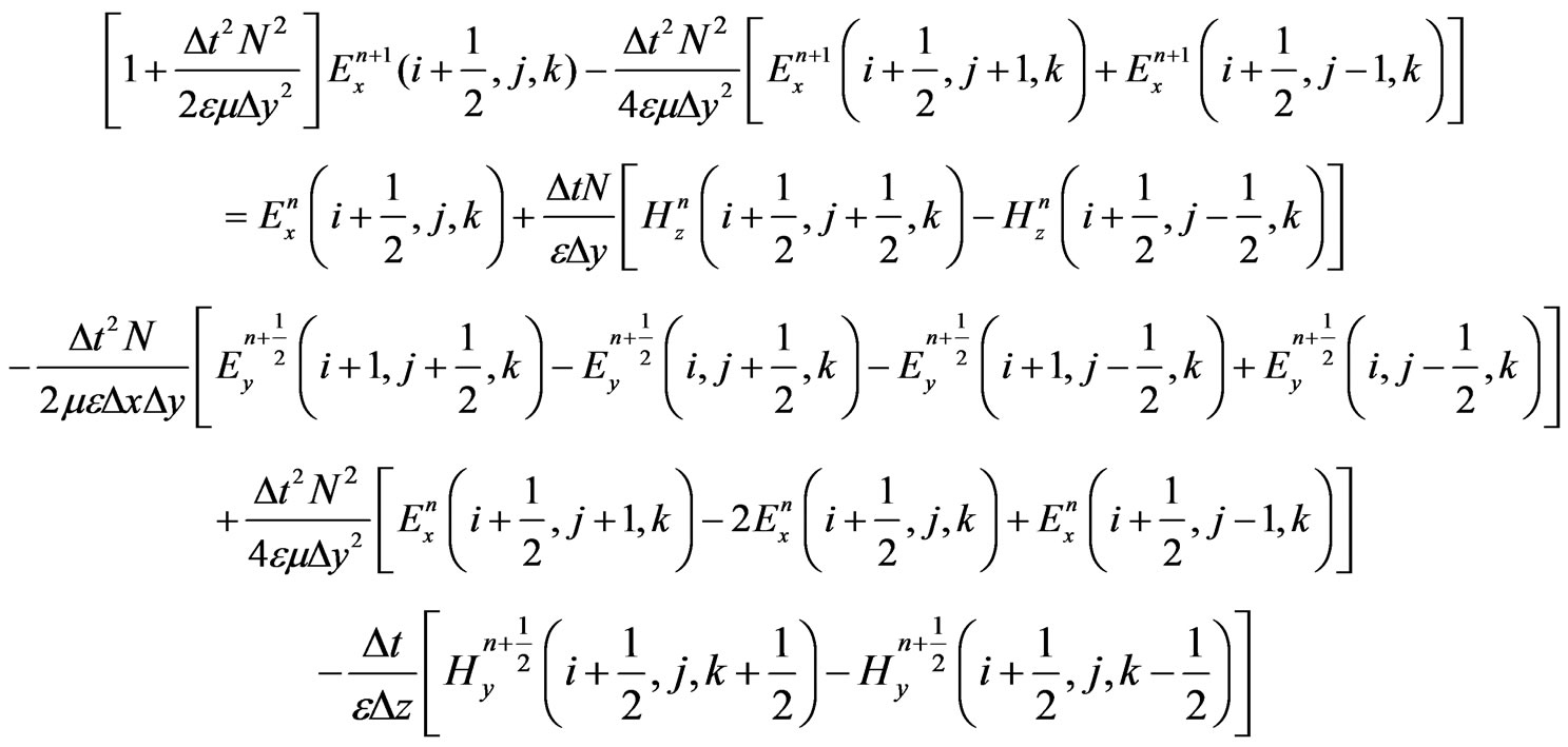 (7)
(7)
Similarly, updating of  component needs the unknown
  component at the same time-step. Substituting Equation (6) into Equation (4), we obtain the discrete equation for
 field,
 (8)
(8)
Therefore, the field components are updated by using Equations (1), (2), and (5)-(8). Components and
and  are explicitly updated first by using Equations (1) and (2). Then,
  and
and components are updated implicitly by solving the tridiagonal matrix equations by using Equations (7) and (8). After
  and
and are obtained, components
  and
and are explicitly updated straightforward by using Equations (5) and (6).
3. Weakly Conditionally Stability
The relations between field components of Equations (1)(6) can be represented in a matrix form as:

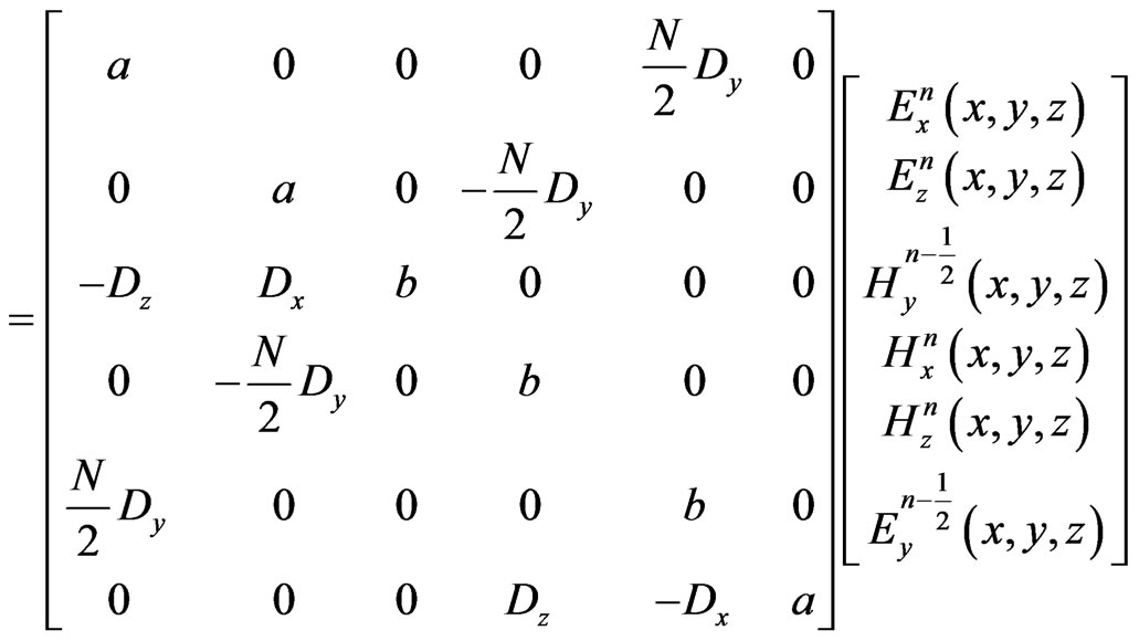 (9)
(9)
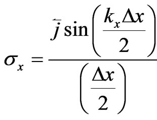
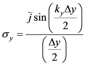
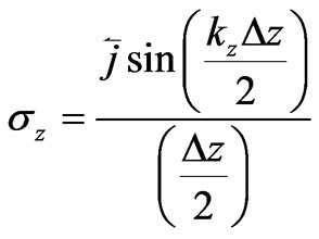
where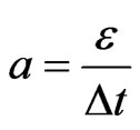 ,
,  ,
,  (
( ) represents the first derivative operator with respect to
 .
.
With no loss of generality, the field components can be written as follows:
 (10)
(10)
 (11)
(11)
where ,
, ,
, .
.

 are wave numbers.
  indicates growth factor.
  are the amplitude of the field components, respectively.
In a discrete space,  can be denoted as:
 (12)
(12)
Then:
 (13)
(13)
 (14)
(14)
 (15)
(15)
where,
 ,
,  ,
,
Substituting these represents into Equation (9), the matrix becomes:
 (16)
(16)
For a nontrivial solution of (16), the determinant of the coefficient matrix in (16) should be zero. It can be obtained:
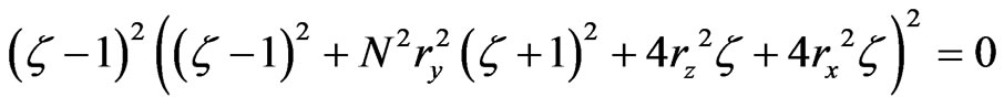 (17)
(17)
where:
 ,
,
 ,
,
 ,
, 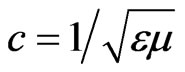
is the speed of light in the medium.
By solving Equation (17), the growth factor  is obtained
 (18)
(18)
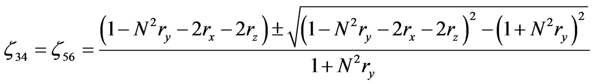 (19)
(19)
To satisfy the stability condition during field advancement, the module of growth factor  can’t be larger than 1. It is evident that the module of
  is unity. For the values of
  and
and , when the condition
  is satisfied,
 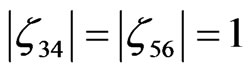 can be obtained. The limitation for time-step size can be calculated as follows:


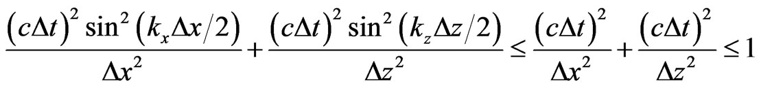 (20)
(20)
This scheme is weakly conditionally stable. The time step is only determined by two space discretizations. The parameter N doesn’t affect the weakly conditionally stability of the HIE-FDTD method.
4. Numerical Dispersion Analysis
We now study the numerical dispersion in the modified HIE-FDTD algorithm. Substitute 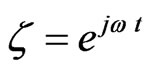 into Equation (16), it can be obtained:
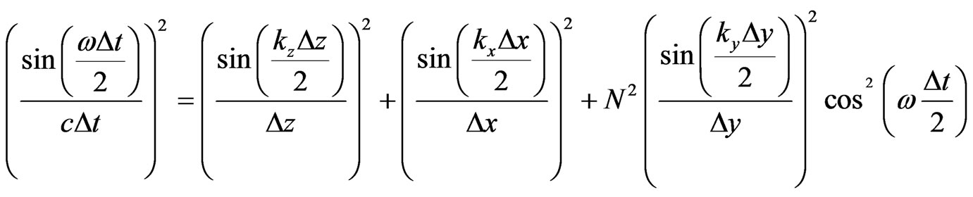 (21)
(21)
For comparison, we take a look at the numerical dispersion relation of the standard HIE-FDTD method.
 (22)
(22)
Compared to the dispersion Equation (22) of the standard HIE-FDTD method, it can be obtained that there is a factor  added to the last term in the right-hand side of the numerical dispersion relations of Equation (21). When a proper value of parameter N is selected, the numerical dispersion of the HIE-FDTD method can be controlled, causing the numerical dispersion to decrease significantly, which is validated in next section.
5. Numerical Validation
Suppose that a wave propagating at angle  and
and  is in the spherical coordinate system. Then,
 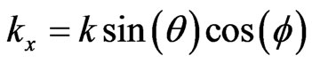 ,
, 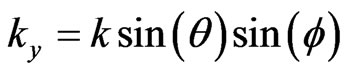 , and
, and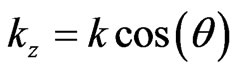 . By substituting them into dispersion relations (21), numerical phase velocity
 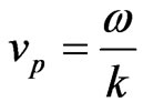 of modified HIE-FDTD method can be solved numerically. To make the discussion simple and easy, only the uniform cell
  is considered here.
  is set to be
 , with
  the operating frequency.
On the  plane
plane . It can be easily seen that the numerical dispersion of modified HIE-FDTD method is the same as that of standard HIE-FDTD method. So we only consider the dispersion performance comparison between the modified HIE-FDTD and standard HIE-FDTD method on other planes.
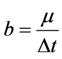
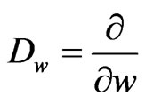
Figures 1-4 show the normalized phase velocities with respect to angle for different CFLN values.
  is set as 45° and 90° respectively. The CFLN is defined as the ratio of the time-step size and the maximum time-step size satisfied with the 3-D CFL condition of conventional FDTD method. Parameter N equal to 1 represents the normalized phase velocity of standard
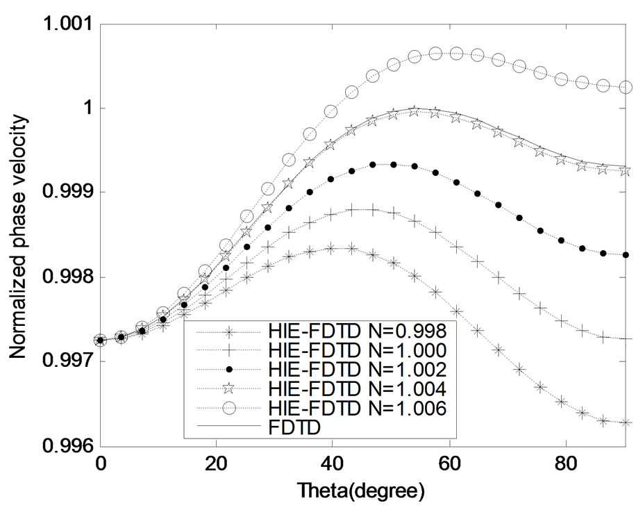
Figure 1. When CFLN = 1, the normalized phase velocities with respect to angle  for different parameter N (
 45°).
45°).
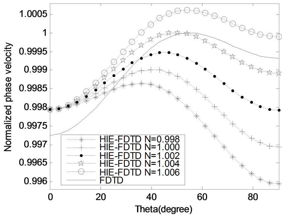
Figure 2. When CFLN = 1.2, the normalized phase velocities with respect to angle  for different parameter N (
 45°).
45°).
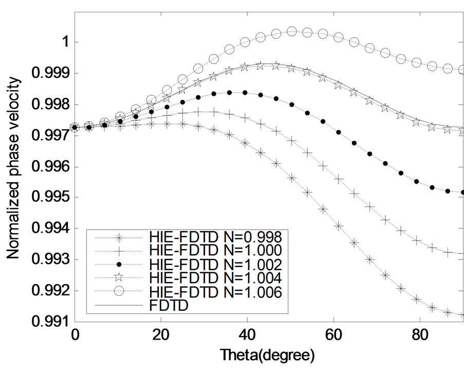
Figure 3. When CFLN = 1, the normalized phase velocities with respect to angle  for different parameter N (
 90°).
90°).
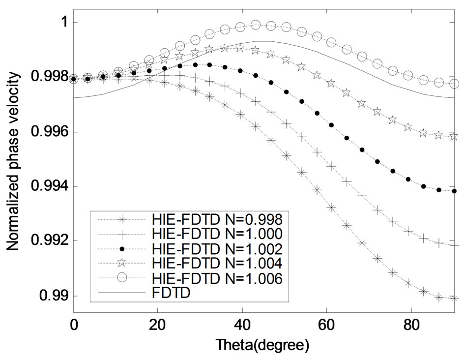
Figure 4. When CFLN = 1.2, the normalized phase velocities with respect to angle  for different parameter N (
 90°).
90°).
HIE-FDTD method. For comparison, the normalized phase velocity of conventional FDTD method is also plotted in these figures.
It can be seen from these figures that the numerical dispersion error of the standard HIE-FDTD (N=1.000) scheme is larger than that of the conventional FDTD method, especially when  is close to 90°. When CFLN = 1.2, the dispersion error along the y axis (
 90°,
90°, = 90°) of standard HIE-FDTD method is almost 4 times as that of conventional FDTD method.
For the modified HIE-FDTD method, the dispersion error is reduced as the value of parameter N increase. Under the CFLN = 1, with N = 1.004, the normalized phase velocities of the modified HIE-FDTD is almost the same as that of the conventional FDTD method for both  45° and
  90° planes. Apparently, the dispersion performance of HIE-FDTD method can be controlled by selecting parameter N.
However, when the value of N exceeds the value 1.004, the normalized phase velocities will exceed 1, which is not the performance we expect. So, select a proper value for parameter N is the key factor for reducing the dispersion error of HIE-FDTD method. It can be easily decided by Equation (22) numerically.
6. Conclusions
A parameter optimized HIE-FDTD method is presented in this letter. The parameter is introduced to minimize the dispersion error. The stability analysis shows that this algorithm is also weakly conditionally stable. Numerical experiments show that this algorithm can dramatically reduce the dispersion error without introducing additional computational cost.
7. Acknowledgements
This work was supported by National Natural Science Foundations of China (No. 61001039 and 60501004), and also supported by the Research Fund for the Doctoral Program of Higher Education of China (20090201120030).
REFERENCES
- K. S. Yee, “Numerical Solution of Initial Boundary Value Problems Involving Maxwell’s Equations in Isotropic Media,” IEEE Transactions on Antennas and Propagations, Vol. 14, No. 5, May 1966, pp. 302-307.
- A. Taflove, “Computational Electrodynamics,” Artech House, Norwood, 1995.
- J. Chen and J. Wang, “A 3-D Hybrid Implicit-Explicit FDTD Scheme with Weakly Conditional Stability,” Microwave and Optical Technology Letters, Vol. 48, No. 3, March 2006, pp. 2291-2294. doi:10.1002/mop.21898
- M. Wang, Z. Wang and J. Chen, “A Parameter Optimized ADI-FDTD Method,” IEEE Antennas and Wireless Propagation Letters, Vol. 2, No. 2, February 2003, pp. 118-121. doi:10.1109/LAWP.2003.815283