Natural Resources
Vol.3 No.2(2012), Article ID:20227,10 pages DOI:10.4236/nr.2012.32009
Monitoring of Net Primary Production in California Rangelands Using Landsat and MODIS Satellite Remote Sensing
![]()
1NASA Ames Research Center, Moffett Field, USA; 2Henan University, College of Environment and Planning, Kaifeng, China; 3CASA Systems 2100, Los Gatos, USA; 4California State University Monterey Bay, Seaside, USA.
Email: christopher@casa2100.com
Received February 29th, 2012; revised April 9th, 2012; accepted April 18th, 2012
Keywords: Grasslands; MODIS; Landsat; California; Net Primary Production
ABSTRACT
In this study, we present results from the CASA (Carnegie-Ames-Stanford Approach) model to estimate net primary production (NPP) in grasslands under different management (ranching versus unmanaged) on the Central Coast of California. The latest model version called CASA Express has been designed to estimate monthly patterns in carbon fixation and plant biomass production using moderate spatial resolution (30 m to 250 m) satellite image data of surface vegetation characteristics. Landsat imagery with 30 m resolution was adjusted by contemporaneous Moderate Resolution Imaging Spectroradiometer (MODIS) data to calibrate the model based on previous CASA research. Results showed annual NPP predictions of between 300 - 450 grams C per square meter for coastal rangeland sites. Irrigation increased the predicted NPP carbon flux of grazed lands by 59 grams C per square meter annually compared to unmanaged grasslands. Low intensity grazing activity appeared to promote higher grass regrowth until June, compared to the ungrazed grassland sites. These modeling methods were shown to be successful in capturing the differing seasonal growing cycles of rangeland forage production across the area of individual ranch properties.
1. Introduction
Due to their unique climate and topography, pastures and rangelands on the Central California coast require continual monitoring for grazing impacts on native plant communities, soil erosion, riparian zones, and water quality. Monitoring of monthly grass production over several years can lead to improved estimates of residual dry matter (RDM) remaining on the soil surface, which is a key indicator of sustainable rangeland management [1,2]. Regular measurements of herbaceous net primary production (NPP) and RDM can help land managers to optimize both plant species composition and forage production to support livestock grazing operations on coastal rangelands.
Mediterranean grasslands cover over 10 million hectares of California’s coastal and inlands foothill regions [3]. The current vegetation is dominated by introduced annual grasses, whereas the original native cover was dominated by perennial bunchgrasses that were intolerant of heavy grazing by livestock [2]. Herbaceous plant growth is generally limited by declines of soil moisture in the summer and by cool temperatures in the winter. The annual production pattern for coastal grasses is rapid growth in the late fall (November) after the first rains have returned, slow winter growth (December-February), and rapid growth again in spring (March-May).
Livestock producers on the California coast have had to adapt to large year-to-years variations in forage quantity and quality. Production and composition of annual-graminoid dominated grasslands are controlled primarily by weather (mainly precipitation patterns) and site conditions (such as elevation, slope, and aspect), and do not respond beneficially to intensive grazing management [1]. In this study, we described the combined use of satellite image analysis and plant production modeling to develop rapid, relatively low-cost grasslands monitoring systems for the California Central Coast. The objectives of the study were to quantify seasonal growing cycles and assess sources of variation in rangeland forage production across the area of individual ranch properties.
2. Site Descriptions
The main study area was central Pacific coastal region near Big Sur, CA (Figure 1). The region has a Mediterranean climate of warm, dry summers and cool, wet winters, with localized summer fog near the coast [4]. Average annual rainfall varies from 40 to 152 cm throughout the region, with highest amounts falling on the higher mountains in the northern extreme of the study area during winter storms. During the summer, fog and low clouds are frequent along the coast. Mean annual temperature is about 10.0˚C to 14.4˚C, from shaded canyon bottoms to exposed ridge tops, respectively. Cattle and sheep ranching began in these coastal grasslands in the 1820 s [5]. Three ranch sites with more than 100 years of differing management history were selected for this study: Brazil Ranch, El Sur Ranch, and Creamery Meadow (formerly South Ranch), with location coordinates and other attributes shown in Table 1.
The Brazil Ranch is located approximately 32 km south of Monterey and covers 490 ha. During the past 100 years, the ranch was actively managed for cattle and horses. After the property was proposed for multiple-unit residential development, Brazil Ranch was purchased by the conservation community with public funding in 2002 to protect its scenic and other natural resource values. In September 2002, the Ranch officially passed to the Unites States Forest Service. The El Sur Ranch is located 10 km south of the Brazil Ranch. This of 7000 acre (2832 ha) private ranch extends north and south along either side of Highway One and includes approximately 108 ha of irrigated pasture for cattle grazing.

Figure 1. Study sites near Big Sur, in the central coastal region of California. The background map derives from 2006 NLCD land cover types.

Table 1. Summary of characteristics of the selected ranch study sites near Big Sur, CA.
Creamery Meadow was originally part of the South Ranch, which is contiguous with The El Sur Ranch property. The South Ranch, comprised of 3620 ha, was originnally granted to Juan Bautista Alvarado by the Mexican government in 1834. After more than 100 years of livestock farming and cheese making, the Ranch was sold by the Molera family to the Nature Conservancy in 1968 on the condition that it would not be developed. The property became Andrew Molera State Park in 1972. No livestock grazing has occurred for more than 40 years on the Creamery Meadow. Low woody shrubs have encroached into marginal areas of the open herbaceous cover at this site.
3. Data Sets
3.1. Meteorological Data
An automatic weather station (Campbell model CR800 data logger) was deployed at Brazil Ranch in late 2007. Hourly data recorded included air temperature, humidity, wind speed, precipitation, and solar radiation.
3.2. Satellite Remote Sensing Data
Cloud-free Landsat 5 TM images (path 43/row 35) were identified and acquired for this study (Table 2). Seasonal images were acquired for the years 2006 to 2009 to represent both wet and dry seasons of the Mediterranean climate. Monthly TM images were acquired for the year 2010. TM bands for the near-infrared (NIR) and red wavelengths were converted into apparent radiance and then at-sensor reflectance using instrument gains and offsets. The MODTRAN4 model was further used for atmospheric correction [6].
The corrected TM bands were used for calculation of the normalized difference vegetation index (NDVI), according to the following equation: NDVI = (NIR – RED)/(NIR + RED). Live, dense vegetation will have a high NIR reflectance and a low red band reflectance, and hence a high NDVI value [7]. As herbaceous cover turns brown, NIR reflectance will decline and red reflectance will increase rapidly.
Landsat NDVI is a widely used remote sensing product to monitor the growth status of herbaceous plant cover [8-10]. This index not only highlights the most densely covered vegetated areas of an image, but can serve as a quantitative input variable to carbon cycle modeling [11]. A close correlation between the VI and NIR values, and especially one that does not saturate at high VI values across many image pixels, indicates that a change in NIR reflectance is sensitive to vegetation cover changes even at relatively high biomass levels for a given ecosystem.
Data products from the Moderate Resolution Imaging Spectroradiometer (MODIS) were acquired at 16-day interval from 2006 through 2010 for the study area. The MODIS MOD13Q1 product was obtained from the Oak Ridge National Laboratory Distributed Active Archive Center. In addition to NDVI at 250 m spatial resolution, MOD13Q1 collection 5 Enhanced Vegetation Index (EVI) products were obtained from atmospherically corrected bi-directional surface reflectances that have been masked for water, clouds, heavy aerosols, and cloud shadows [12].
EVI was developed to optimize the greenness signal, or area-averaged canopy photosynthetic capacity, with improved sensitivity in high biomass regions. EVI has been found useful in estimating absorbed photosyntheically active radiation (PAR) related to chlorophyll contents in vegetated canopies [13] and has been shown to be highly correlated with processes that depend on absorbed light, such as gross primary productivity (GPP) [14,15].
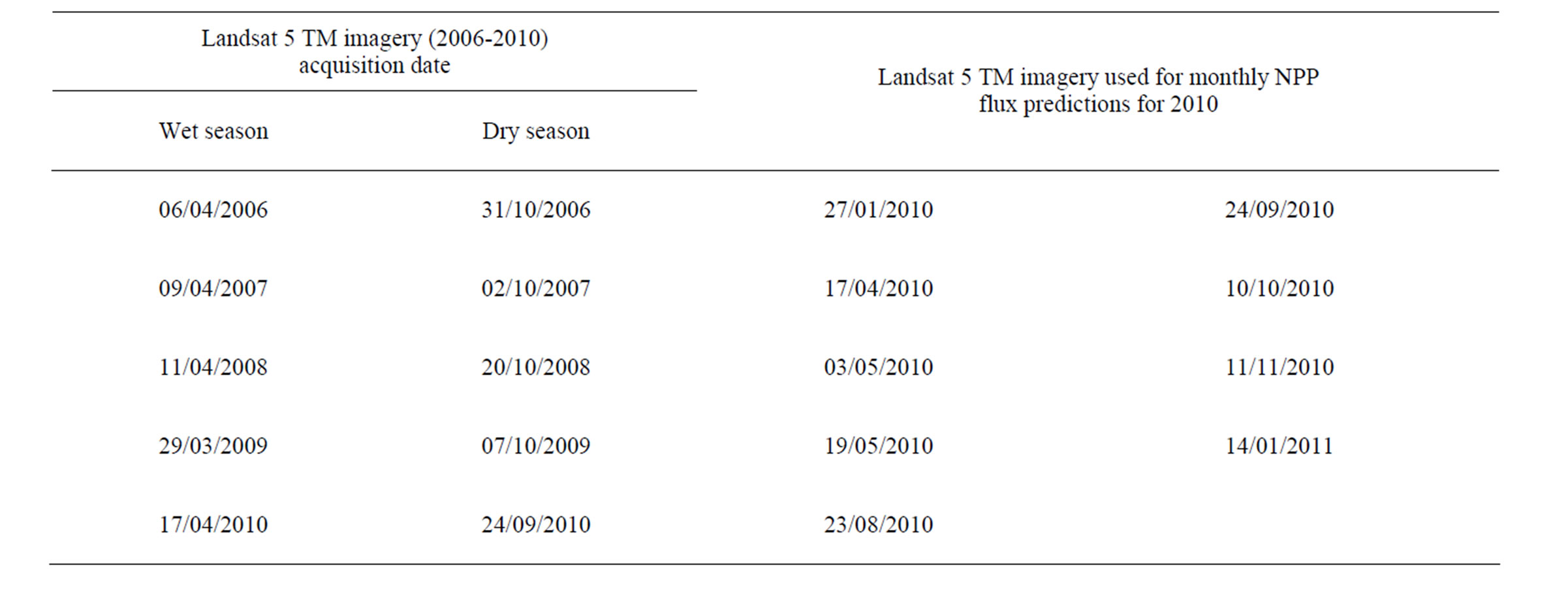
Table 2. List of Landsat 5 TM images acquired for CASA model NPP predictions.
4. Modeling Methodology
As thoroughly documented in previous publications [16,17], the monthly NPP flux, defined as net fixation of CO2 by vegetation, is computed in the modeling system called CASA Express on the basis of light-use efficiency. Monthly production of plant biomass is estimated as a product of time-varying surface solar irradiance (Sr), and EVI from the Landsat or MODIS satellites, plus a constant light utilization efficiency term (emax) that is modified by time-varying stress scalar terms for temperature (T) and moisture (W) effects:

The emax term was set uniformly at 0.55 g C MJ–1 PAR, a value that derives from calibration of predicted annual NPP to previous field estimates [17]. This model calibration has been validated globally by comparing predicted annual NPP to more than 1900 field measurements of NPP [18,19]. The T stress scalar is computed with reference to derivation of optimal temperatures (Topt) for plant production. The W stress scalar is estimated from monthly water deficits, based on a comparison of moisture supply (precipitation and stored soil water) to potential evapotranspiration (PET) demand using the method of Thornthwaite [20].
The 2001 National Land Cover Dataset (NLCD) 30 m map from the U.S. Geologic Survey was aggregated to 250 m pixel resolution and used to specify the predominant land cover class for the W term in each pixel. The NLCD product was derived from 30 m resolution Landsat satellite imagery and has been shown to have a high level of accuracy in the western United States [21]. Monthly mean surface solar flux, air temperature and precipitation for model simulations over the years 2007-2010 came from the Brazil Ranch weather station record. Soil settings in the model for texture classes (fine, medium and coarse) and depth to bedrock for maximum plant rooting depths were assigned to the USDA STATSGO data set.
In order to examine monthly NPP patterns of California grasslands at the landscape scale (several km2), MODIS EVI datasets were supplemented with Landsat NDVI layers as direct inputs to the CASA Express model. As a consequence, predicted monthly NPP flux at 30 m resolution was generated from addition of cloud free Landsat imagery. Nine Landsat scenes for 2010 were used in this study to predict NPP fluxes layers in central coast region of California (Table 2).
5. CASA NPP Validation for California Grasslands
Validation of NPP predicted by CASA Express for California grasslands was carried out using measured CO2 fluxes from the nearest Ameriflux tower site (Heinsch et al., 2006), the Tonzi Ranch study site (38˚ 24.40 N, 120˚ 57.04 W, at 129 m elevation) located 245 km northeast of Big Sur. This site was an oak-grass savanna consisting of scattered blue oak trees (Quercus douglasii), with occasional gray pine trees (Pinus sabiniana L.), and grazed grassland (Brachypodium distachyon L., Hypochaeris glabra L., Bromus madritensis L. and Cynosurus echinatus L.). Trees cover 40% of the landscape [22]. Grass grows from November to May, after which it senesces rapidly.
Much like the Big Sur coast, climate at the Tonzi Ranch site is Mediterranean with a mean annual temperature of 16.3˚C and total annual precipitation of 56 cm. The soil is an Auburn type, extremely rocky silt loam (Lithic haploxerepts) composed of 43% sand, 43% silt and 13% clay. Volumetric water content (VWC) at 50 cm soil depth peaks at 35% - 40% in the wet season months (NovMay) and drops to 15% - 20% in the dry summer months (Jun-Oct).
Carbon dioxide fluxes, water vapor, and meteorological variables were measured continuously at Tonzi Ranch for several years using eddy covariance systems. Monthly gross primary productivity (GPP) was calculated based on year-round tower flux measurements [23]. Baldocchi et al. [22] reported that grasslands at Tonzi Ranch typically stopped transpiring when VWC of the soil dropped below 15% in early summer. Oak trees, on the other hand, were able to continue to transpire into the summer months, albeit at low rates, under very dry soil conditions (nearly 10% VWC). Compared to grass cover, trees at the site were able to endure such low water potentials and maintain basal levels of carbon metabolism because tree roots were able to access sources of water in the soil unavailable to grass roots.
In a comparison study of standard MODIS algorithms for primary production to the Tonzi Ranch tower flux record, Heinsch et al. [24] reported that the standard MODIS algorithms failed to capture all seasonal dynamoics. Although standard MODIS algorithms could capture the seasonal onset of growth during the wet season as well as the return of the rainy season in November, they failed to capture the changes in production during the late summer when the site was extremely water limited. From this, the authors concluded that standard MODIS production algorithms failed to account for vegetation communities that had drought tolerance adaptations, (as documented by [22]) in this California Mediterranean climate.
Consequently, for CASA Express model applications in rangelands of California (for which Tonzi Ranch is the only tower site reporting carbon flux data), we made an adjustment in the available water storage content for the deeper rooting layer of shrubs and trees that may be present at such sites. This adjustment made available 80% more VWC for transpiration by shrubs and trees than is commonly set for other moist forested climate zones of the western United States. The nine closest MODIS EVI 250 m pixel values to the center tower location were extracted for these NPP validation outputs and combined as monthly average NPP from 2005 to 2007. The only model input data set to CASA Express for these Tonzi Ranch runs that differed from Big Sur runs that follow were monthly mean climate grids, which came from 4 km spatial resolution PRISM products [25] for the Tonzi Ranch location.
AmeriFlux eddy-correlation data sets were obtained from the central data repository located at the Carbon Dioxide Information Analysis Center (CDIAC; http://public. ornl.gov/ameriflux/dataproducts.shtml). Level 4 AmeriFlux records contained gap-filled and ustar filtered records, complete with calculated gross productivity on varying time intervals including hourly, daily, weekly, and monthly with flags for the quality of the original and gap-filled data. Monthly NPP fluxes were computed from Level 4 estimates of gross primary production (GPP) by adjustment within an uncertainty range of 40% - 50% of GPP carbon flux for temperate ecosystems [26,27].
Observed tower fluxes and CASA Express predicted monthly NPP fluxes were significantly correlated across all seasons of the Tonzi Ranch measurement period, with a coefficient of determination (R2) of 0.89 and root mean square error (RMSE) of 8.8 g C m–2 (Figures 2 and 3). Tower measurements adjusted to 40% GPP matched better with CASA NPP than 50% GPP tower approximations.
CASA predicted peak summer NPP fluxes in 2007 were notably lower than the estimated tower flux values. This may have been related to extreme drought tolerance of the mixed savanna ecosystem under the low precipitation amounts recorded in 2007, compared to the previous two years [25].
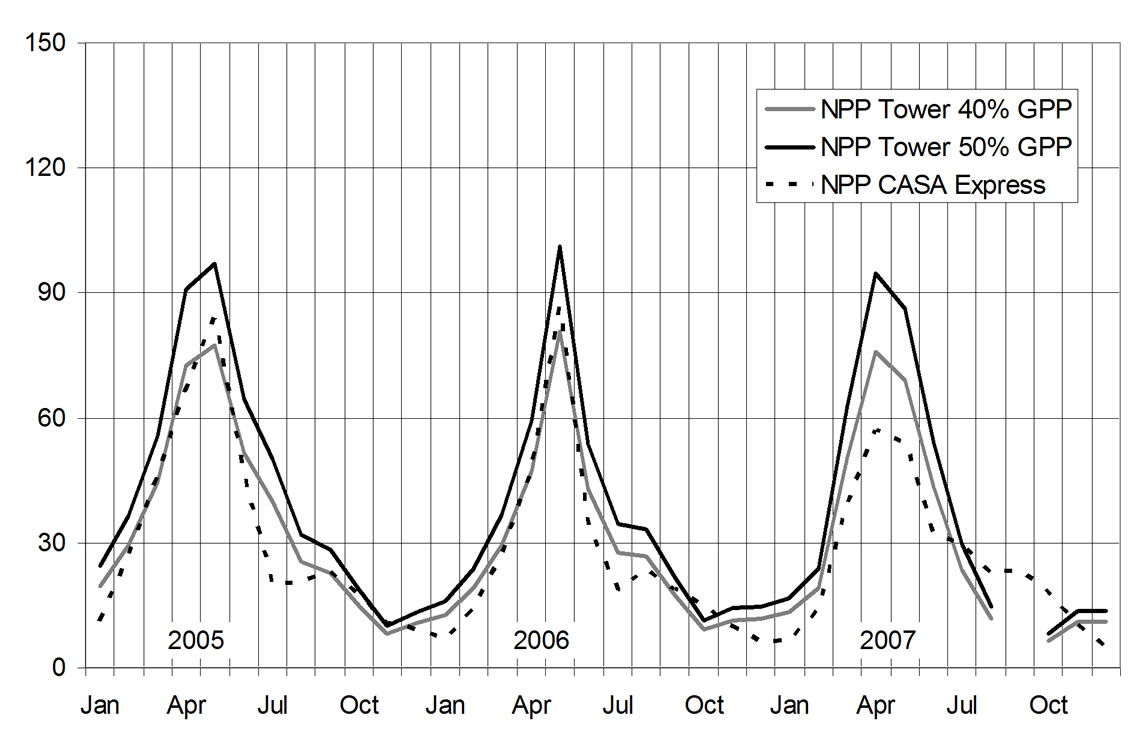
Figure 2. Comparison of CASA NPP predictions (mean value of 250-m pixel outputs, n = 9) with monthly aggregated Tonzi Ranch tower flux measurements from 2005 to 2007. Units are g C m–2 mo–1.
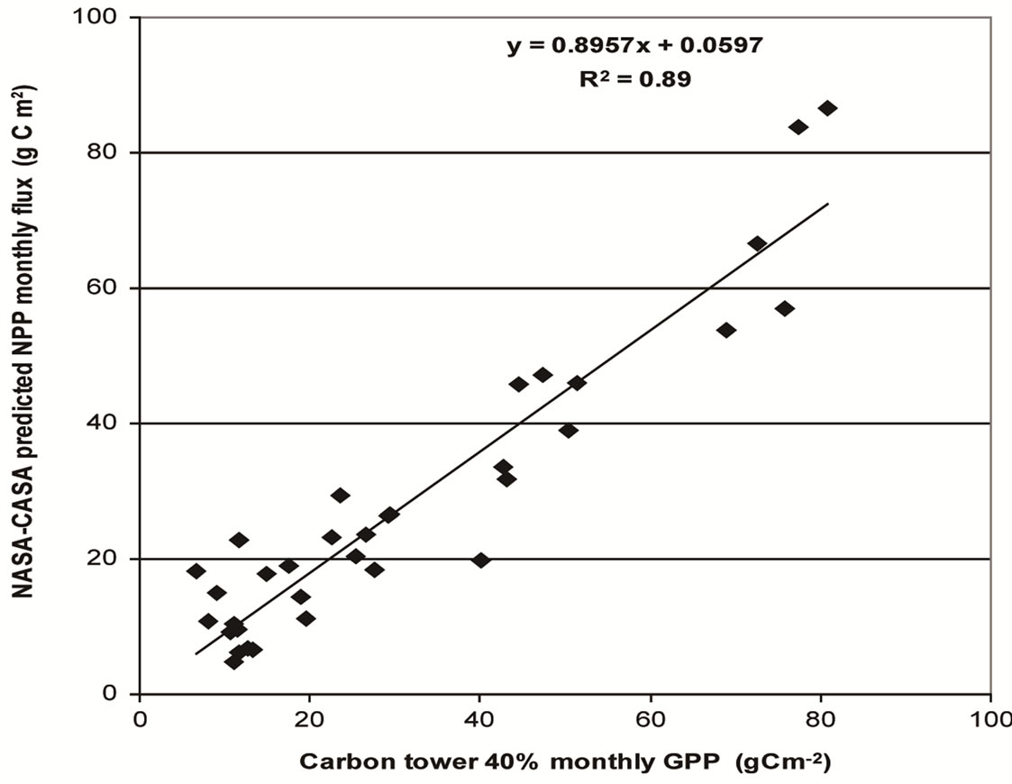
Figure 3. Scatter plot of monthly flux tower measurements at Tonzi Ranch (2005-2007) versus CASA Express model outputs, both from Figure 2.
6. Results
6.1. Reflectance Band Comparisons
To understand seasonal variability of herbaceous plant growth at the three Big Sur grassland sites, we first plotted 16-day average reflectance and standard error values for 2010 of MODIS red, NIR, and blue bands (Figure 4). Averaged NIR reflectance increased strongly at around Julian day 50 (February 19) until peak levels of NIR reflectance were observed by Julian day 121 (May 1) in 2010. The averaged red band reflectance began to increase strongly at Julian day 153 (June 2) until peak levels were observed at Julian day 185 (July 4). The MODIS blue band reflectance was relatively constant year-round. Together, these changes in NIR and red band reflectance indicated an active grassland growing season from mid-February to late May, followed by a relatively dormant season from June through the end of January.
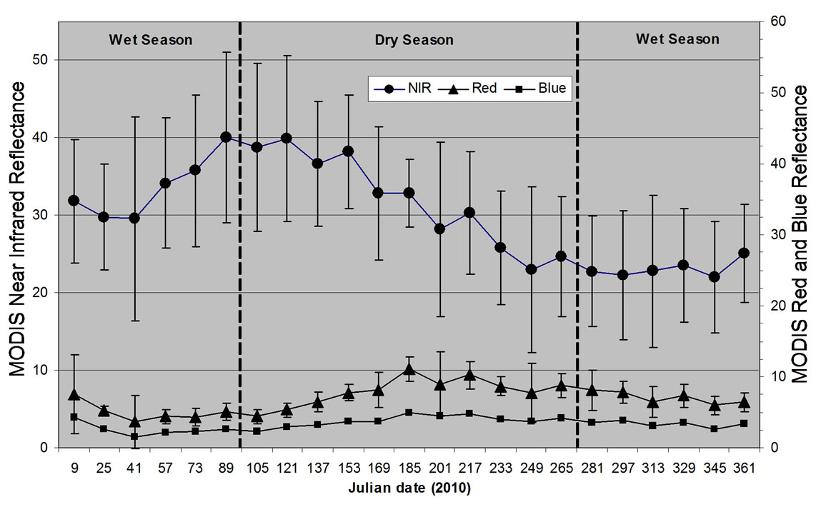
Figure 4. Averaged reflectance and standard error values of the MODIS bands used for EVI and NDVI calculations in the 2010 16 day MOD13Q1 product (n = 34 combined 250 m grassland pixels from the three Big Sur study sites).
Five years (2006-2010) of seasonal average reflectances of MODIS NIR and red bands revealed more dense grassland cover development during the growing seasons of 2009 and 2010 than during the three previous years (Figure 5). In general, standard deviation values of the NIR reflectances were slightly higher in wet seasons than in the dry seasons, due presumably to the higher frequency of cloud cover from major winter storm systems.
6.2. Comparison of MODIS and Landsat VIs
We plotted the past five years (2006-2010) of average Landsat NDVI, MODIS NDVI and MODIS EVI for the three study sites together (Figure 6) to compare sensor VI variability. Landsat NDVI followed the same overall inter-annual patterns as MODIS VIs, showing again that the growing seasons of 2009 and 2010 supported higher herbaceous cover density that did the three previous years. Precipitation amounts recorded at the nearby Big Sur Station gauge confirmed that 2007 was 50% drier than 2009 and 2010, and that 2008 was nearly 25% drier than these two subsequent wet seasons (Figure 6). Landsat NDVI was less sensitive than either MODIS NDVI or MODIS EVI to these moisture shortage conditions in the wet season of 2007.
However, Landsat bands provide inherently more detailed vegetation information (at 30 m resolution) per site than is possible with MODIS (250 m resolution) VIs, as reflected in the larger standard errors in the mean Landsat NDVI values compared to MODIS standard errors. Except for the wet season of 2007, all the other standard error values of Landsat NDVI are larger than the corresponding MODIS NDVI (Figure 6).
For calibration of CASA to use an EVI input range, we computed relatively stable ratios of around 0.71 in the wet season and 0.55 in dry season between MODIS EVI and MODIS NDVI over the years 2006-2010 (Table 3). The standard deviations of the ratio between MODIS NDVI and MODIS EVI were 0.04 and 0.02 in the wet and dry seasons, respectively. The standard deviations of the ratio between MODIS EVI and Landsat NDVI were found to be slightly higher at 0.05 and 0.03 in the wet and dry seasons, respectively, over the five years.
A comparison of 16-day time series data among the three grassland sites showed the El Sur Ranch site to have the highest mean MODIS EVI values in all seasons (Figure 7). Even in the relatively dry years of 2007 and 2008, the irrigated pastures on El Sur Ranch remained higher in EVI on average than did the grass cover at Brazil Ranch and Creamery Meadow during their peak green periods of 2009 and 2010. During the relatively dry years of 2007 and 2008, EVI at the ungrazed Creamery Meadow site with its sparsely mixed shrub cover remained higher during the summer and autumn periods than did corresponding EVI values at Brazil Ranch.
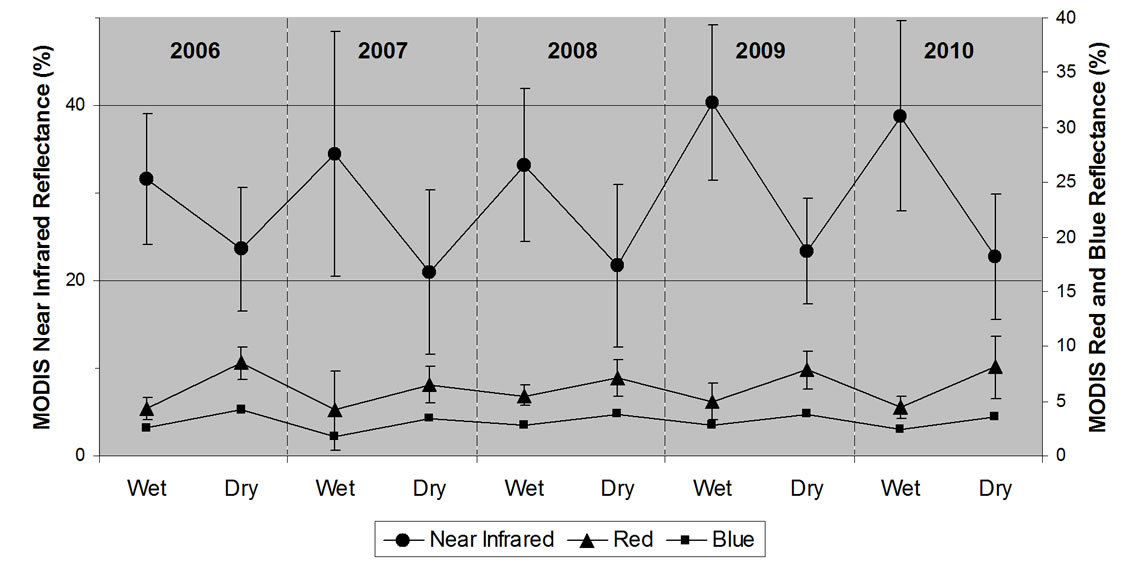
Figure 5. Averaged seasonal (wet and dry seasons) reflectance and standard error values of the MODIS bands used for EVI and NDVI calculations in the 2006-2010 MOD13Q1 product (n = 34,250 m grassland pixels from the three Big Sur study sites).

Figure 6. Averaged MODIS EVI and NDVI (n = 34), and Landsat NDVI (n = 2001, Standard Error bars in white) for wet and dry seasons across grassland sites in central coast region of California (2006-2010).

Table 3. Variation in the mean seasonal ratios between EVI and NDVI for Big Sur grassland sites.
It is important to note that MODIS EVI incorporates features that NDVI does not, particularly from the Atmospherically Resistant Vegetation Index (ARVI; [28]) and the Soil-Adjusted Vegetation Index (SAVI; [29]) to reduce atmospheric and soil background influences. Since Landsat NDVI and MODIS EVI values were both highly correlated with their reflectance in the NIR bands (Figure 8), ratios of the two VIs were computed (Table 4) and applied to corresponding Landsat scenes. These data sets became the 30 m adjusted EVI values that were input to CASA Express for 2010 monthly NPP flux calculations across all three grassland sites.
6.3. Predicted NPP Flux of Grassland Sites
During all of 2010, predicted NPP flux of pastures on the El Sur Ranch was higher on average than NPP on the other two sites (Figure 9). Peak monthly NPP predicted in April (at all sites) was 30% higher on the El Sur Ranch than peak monthly NPP predicted for unmanaged Creamery Meadow. Peak monthly NPP predicted for Brazil Ranch grasslands was 15% higher on average than peak monthly NPP predicted for Creamery Meadow, whereas the dry season (August-September) NPP predicted for Creamery Meadow was higher on average than dry season NPP predicted for Brazil Ranch.
Predicted annual NPP flux pastures on the El Sur Ranch in 2010 was 448 g C m–2, while predicted annual NPP for Brazil Ranch and Creamery Meadow averaged 311 g C m–2 and 303 g C m–2, respectively. Grazing activeity at Brazil Ranch appeared to promote higher grass regrowth until June, compared to the ungrazed Creamery Meadow (Figure 9). Irrigation of pastures on the El Sur Ranch explained higher year-round NPP compared to unirrigated Brazil Ranch.
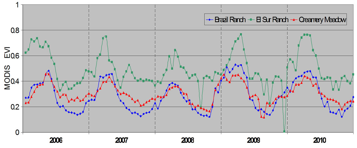
Figure 7. Averaged MODIS EVI time series profiles (2006- 2010) at 250 m resolution for the three grassland sites based on pixel numbers shown in Table 1.

Figure 8. Comparison between MODIS EVI and Landsat NDVI and their respective near-infrared reflectances for nine dates in 2010 and 2011 across all three study sites near Big Sur. The closer match of MODIS EVI to the 1:1 lines (than that of Landsat NDVI) implied that adjustment of Landsat NDVI to track MODIS EVI could minimize saturation of wet season VI inputs to CASA Express model runs at 30 m resolution.

Table 4. Averaged ratios of MODIS EVI to Landsat NDVI in 2010 for Big Sur grassland sites.

Figure 9. Predicted mean monthly NPP for 2010 at the three grassland sites based on 30 m resolution pixel numbers shown in Table 1.
One standard error of the mean monthly predicted NPP flux was plotted in Figure 10 to capture 30 m resolution detail resulting from Landsat inputs to the model. This plot revealed important landscape-level variations among sites. For example, Creamery Meadow showed the highest spatial variation across all seasons in 2010, which could be related to some encroachment by woody shrub cover during the past fifty years. Less intensive and more random grazing on the Brazil Ranch pastures may explain, in part, the higher variation in monthly NPP flux in wet season than in dry season, compared to the El Sur Ranch site.
A closer examination of the CASA Express results for Brazil Ranch in 2010 showed the strong effects of topography and soil development on predicted forage NPP (Figure 11). Areas of lowest herbaceous biomass production were located on the steepest south-facing slopes which (based on aerial imagery of several meters resolution from the National Agriculture Imagery Program-NAIP), included small landslide activity. Other areas of relatively low NPP were identified on ridge-top plateaus with exposed rocky outcrops. Deep soil development in these areas was observed to be rare, leading to extreme moisture and heat stress on any plants that may begin to colonize these locations.
7. Discussion
The outcome of a well-managed grazing system should be to increase herbaceous production by ensuring that forage species can capture sufficient resources (e.g., light,

Figure 10. Standard errors of 2010 mean monthly NPP flux at the three grassland sites.

Figure 11. Monthly NPP flux in 2010 predicted by CASA Express for grassland cover at the Brazil Ranch in April and in October. Inset shows Ranch boundary lines with grassland coverage shaded.
water, and nutrients) to promote growth and by enable livestock to harvest available forage more efficiently [30]. The potential for grazing to increase plant production may be explained in the grazing optimization hypothesis, which states that primary production increases above that of ungrazed vegetation as grazing intensity increases to an optimal level, followed by a decrease at greater grazing intensities [31]. However, grazing was observed to increase primary production in only about 20% of the case studies evaluated globally [32,33]. Increases in forage with grazing therefore are associated with systems that allow for sufficient periods of recovery following intensive herbivory [33]. In fact, the pattern required to increase primary production of forage resembles that of rangelands that support herds of migratory herbivores, which have a period of intensive early-season grazing, followed by a longer period of low intensity grazing [34].
There have been several experimental studies of the effects of grazing on carbon cycles of grasslands in the western United States, leading to somewhat different conclusions. Schuman et al. [35] reported that twelve years of grazing under different stocking rates did not change the total masses of C and N in the plant-soil (0 - 60 cm) system but did change the distribution of C and N among the system components, primarily via a significant increase in the masses of C and N in the root zone (0 - 30 cm) of the soil profile. Hayes and Holl [36] reported that native grass cover did not differ significantly between grazed and ungrazed grassland sites on the California coast, but species richness of native perennial forbs was higher in ungrazed sites.
The combined remote sensing and modeling methods presented in this paper can uniquely capture the differing seasonal growing cycles of rangeland forage production across the area of individual ranch properties. By way of example, if it can be assumed that cattle move randomly across the pasture sites and consume the same amount of grass forage biomass during each month, we can estimate the potential plant production improvement by low-intensity grazing activity on coastal California rangelands. In the most conservative terms, this is equivalent to the difference in NPP during the wet season between a grazed rangeland (Brazil Ranch) and ungrazed grassland (Creamery Meadow). Based on 2010 results (Figure 9), the carbon flux value of improvement from grazing activity on Brazil Ranch was 23 g C m–2, which is equivalent to 7% of annual NPP at this site. Since the satellite imagery can provide an averaged estimate of herbaceous green cover for any given month, rather than a cumulative change over the entire grazing period, we were unable to directly estimate the amount of forage biomass consumed by cattle on Brazil Ranch. That additional forage biomass produced and consumed by livestock could conceivably double the carbon flux value of improvement from low intensity grazing activity at the site.
In conclusion, satellite remote sensing together with NPP modeling methods were shown to capture the differing seasonal growing cycles of rangeland forage production across ranch properties on the central California coast. With further development, these CASA Express methods can provide continual and standardized monitoring indices of grazing and irrigation impacts on RDM dynamics and native plant communities for any rangeland in the State.
8. Acknowledgements
This research was supported by an appointment of the first author to the NASA Postdoctoral Program at the NASA Ames Research Center, administered by Oak Ridge Associated Universities through a contract with NASA. The authors are grateful to the US Forest Service, Los Padres National Forest (Ecosystem Manager Jeff Kwasny), for facilitating access to the Brazil Ranch property.
REFERENCES
- J. W. Bartolome, M. C. Stroud and H. F. Heady, “Influence of Natural Mulch on Forage Production on Differing California Annual Range Sites,” Journal of Range Management, Vol. 33, No. 1, 1980, pp. 4-8.
- J. W. Bartolome, W. E. Frost, N. K. McDougald and M. Connor, “California Guidelines for Residual Dry Matter (RDM) Management on Coastal and Foothill Annual Rangelands,” University of California, Division of Agriculture and Natural Resources, Vol. 8092, 2002, 8 p.
- H. F. Heady, T. C. Foin, M .M. Hektner, D. W. Taylor, M. G. Barbour and W. J. Barry, “Coastal Prairie and Northern Coastal Scrub,” Terrestrial Vegetation of California, California Native Plant Society Special Publication, 2nd Edition, Sacramento, 1988, pp. 733-760.
- J. C. Hickman, “The Jepson Manual: Higher Plants of California,” University of California Press, Berkeley, 1993.
- L. T. Burcham, “California Range Land: An HistoricoEcological Study of the Range Resources in California,” Center for Archaeological Research at Davis, University of California, Berkeley, 1957.
- S. M. Adler-Golden, M. W. Matthew, L. S. Bernstein, R. Y. Levine, A. Berk, S. C. Richtsmeier, P. K. Acharya, G. P. Anderson, J. W. Felde, J. A. Gardner, M. L. Hoke, L. S. Jeong, B. Pukall, A. J. Ratkowski and H. K. Burke, “Atmospheric Correction for Short-Wave Spectral Imagery Based on MODTRAN4,” Summaries of the Eighth Annual JPL Earth Science Workshop, Vol. 3753, No. 7, 1999, pp. 61-69. http://jpl.nasa.gov
- R. E. Burgan and R. A. Hartford, “Monitoring Vegetation Greenness with Satellite Data,” US Department of Agriculture, Forest Service, Intermountain Research Station, Ogden, 1993.
- J. B. Campbell, “Introduction to Remote Sensing,” 2nd Edition, The Guilford Press, New York City, 1996.
- J. W. Rouse, R. H. Haas, J. A. Schell and D. W. Deering, “Monitoring Vegetation Systems in the Great Plains with ERTS,” 3rd ERTS Symposium, NASA SP-351, Vol. 1, 1993, pp. 309-317.
- C. J. Tucker, “Red and Photographic Infrared Linear Combinations for Monitoring Vegetation,” Remote Sensing of Environment, Vol. 8, No. 2, 1979, pp. 127-150. doi:10.1016/0034-4257(79)90013-0
- C. S. Potter, J. T. Randerson, C. B. Field, P. A. Matson, P. M. Vitousek, H. A. Mooney and S. A. Klooster, “Terrestrial Ecosystem Production: A Process Model Based on Global Satellite and Surface Data,” Global Biogeochemical Cycles, Vol. 7, No. 4, 1993, pp. 811-841. doi:10.1029/93GB02725
- Oak Ridge National Laboratory Distributed Active Archive Center (ORNL DAAC), “MODIS Subsetted Land products,” 2011. http://daac.ornl.gov/MODIS/modis.html
- A. Huete, K. Didan, T. Miura, E. P. Rodriguez, X. Gao and L. G. Ferreira, “Overview of the Radiometric and Biophysical Performance of the MODIS Vegetation Indices,” Remote Sensing of Environment, Vol. 83, No. 1-2, 2002, pp. 195-213. doi:10.1016/S0034-4257(02)00096-2
- A. F. Rahma, D. A. Sims, V. D. Cordova and B. Z. El-Masri, “Potential of MODIS EVI and Surface Temperature for Directly Estimating Per-Pixel Ecosystem C Fluxes,” Geophysical Research Letters, Vol. 32, 2005, pp. L19404. doi:10.1029/2005GL024127
- X. M. Xiao, Q. Y. Zhang, B. Braswell, S. Urbanski, S. Boles, S. Wofsy, B. Moore III and D. Ojima, “Modeling Gross Primary Production of Temperate Deciduous Broadleaf Forest Using Satellite Images and Climate Data,” Remote Sensing of Environment, Vol. 91, No. 2, 2004, pp. 256-270. doi:10.1016/j.rse.2004.03.010
- C. Potter, P. Gross, V. Genovese and M.-L. Smith, “Net Primary Productivity of Forest Stands in New Hampshire Estimated from Landsat and MODIS Satellite Data,” Carbon Balance and Management, Vol. 2, 2007, p. 9. doi:10.1186/1750-0680-2-9
- C. Potter, S. Klooster, A. Huete and V. Genovese, “Terrestrial Carbon Sinks for the United States Predicted from MODIS Satellite Data and Ecosystem Modeling,” Earth Interactions, Vol. 11, No. 13, 2007, pp. 1-21. doi:10.1175/EI228.1
- C. Potter, S. Klooster, R. Myneni, V. Genovese, P.-N. Tan and V. Kumar, “Continental-Scale Comparisons of Terrestrial Carbon Sinks Estimated from Satellite Data and Ecosystem Modeling 1982-1998,” Global and Planetary Change, Vol. 39, No. 3-4, 2003, pp. 201-213. doi:10.1016/j.gloplacha.2003.07.001
- D. L. Zheng, S. Prince and R. Wright, “Terrestrial Net Primary Production Estimates for 0.5˚ Grid Cells from Field Observations—A Contribution to Global Biogeochemical Modeling,” Global Change Biology, Vol. 9, No. 1, 2003, pp. 46-64. doi:10.1046/j.1365-2486.2003.00534.x
- C. W. Thornthwaite, “An Approach toward Rational Classification of Climate,” Geographic Reviews, Vol. 38, No. 1, 1948, pp. 55-94. doi:10.2307/210739
- J. D. Wickham, S. V. Stehman, J. H. Smith and L. Yang, “Thematic Accuracy of the 1992 National Land-Cover Data for the Western United States,” Remote Sensing of Environment, Vol. 91, No. 3-4, 2004, pp. 452-468. doi:10.1016/j.rse.2004.04.002
- D. D. Baldocchi, L. K. Xu and N. Kiang, “How Plant Functional-Type, Weather, Seasonal Drought, and Soil Physical Properties Alter Water and Energy Fluxes of an Oak-Savanna and an Annual Grassland,” Agricultural and Forest Meteorology, Vol. 123, No. 1-2, 2004, pp. 13-39. doi:10.1016/j.agrformet.2003.11.006
- S. Ma, D. D. Baldocchi, L. K. Xu and T. Hehn, “InterAnnual Variability in Carbon Dioxide Exchange of an Oak/Grass Savanna and Open Grassland in California,” Agricultural and Forest Meteorology, Vol. 147, 2007, pp. 157-171. doi:10.1016/j.agrformet.2007.07.008
- F. A. Heinsch, M. S. Zhao, S. W. Running, J. S. Kimball, and R. R. Nemani, “Evaluation of Remote Sensing Based Terrestrial Productivity from MODIS Using Tower Eddy Flux Network Observations,” IEEE Transactions on Geoscience and Remote Sensing, Vol. 44, No. 7, 2006, pp. 1908-1924. doi:10.1109/TGRS.2005.853936
- C. Daly, M. Halbleib, J. I. Smith, W. P. Gibson, M. K. Doggett, G. H. Taylor, J. Curtis and P. P. Pasteris, “Physiographically-Sensitive Mapping of Temperature and Precipitation across the Conterminous United States,” International Journal of Climatology, Vol. 28, No. 15, 2008, pp. 2031-2064. doi:10.1002/joc.1688
- R. H. Waring, J. J. Landsberg and M. Williams, “Net Primary Production of Forests: A Constant Fraction of Gross Primary Production?” Tree Physiology, Vol. 18, No. 2, 1998, pp. 129-134. doi:10.1093/treephys/18.2.129
- Y. J. Zhang, M. Xu, H. Chen and J. Adams, “Global Pattern of NPP to GPP Ratio Derived from MODIS Data: Effects of Ecosystem Type, Geographical Location and Climate,” Global Ecology and Biogeography, Vol. 18, No. 3, 2009, pp. 280-290. doi:10.1111/j.1466-8238.2008.00442.x
- Y. J. Kaufman and D. Tanré, “Atmospherically Resistant Vegetation Index (ARVI) for EOS-MODIS,” IEEE Transactions on Geoscience and Remote Sensing, Vol. 30, No. 2, 1992, pp. 261-270. doi:10.1109/36.134076
- A. R. Huete, “A Soil-Adjusted Vegetation Index (SAVI),” Remote Sensing of Environment, Vol. 25, No. 3, 1988, pp. 295-309. doi:10.1016/0034-4257(88)90106-X
- D. D. Briske, J. D. Derner, J. R. Brown, S. D. Fuhlendorf, W. R. Teague, K. M. Havstad, R. L. Gillen, A. J. Ash and W. D. Willms, “Rotational Grazing on Rangelands: Reconciliation of Perception and Experimental Evidence,” Rangeland Ecology and Management, Vol. 61, No. 1, 2008, pp. 3-17. doi:10.2111/06-159R.1
- S. J. McNaughton, “Grazing as an Optimization Process: Grass-Ungulate Relationships in the Serengeti,” American Naturalist, Vol. 113, No. 5, 1979, pp. 691-703. doi:10.1086/283426
- A. J. Belsky, “Does Herbivory Benefit Plants? A Review of the Evidence,” American Naturalist, Vol. 127, No. 6, 1986, pp. 870-892. doi:10.1086/284531
- D. G. Milchunas and W. K. Laurenroth, “Quantitative Effects of Grazing on Vegetation and Soils over a Global Range of Environments,” Ecological Monographs, Vol. 63, No. 4, 1993, pp. 327-366. doi:10.2307/2937150
- D. A. Frank and S. J. McNaughton, “Evidence for the Promotion of Aboveground Grassland Production by Native Large Herbivores in Yellowstone National Park,” Oecologia, Vol. 96, No. 2, 1993, pp. 157-161. doi:10.1007/BF00317727
- G. E. Schuman, J. D. Reeder, J. T. Manley, R. H. Hart and W. A. Manley, “Impact of Grazing Management on the Carbon and Nitrogen Balance of a Mixed-Grass Rangeland,” Ecological Applications, Vol. 9, No. 1, 1999, pp. 65-71. doi:10.1890/1051-0761(1999)009[0065:IOGMOT]2.0.CO;2
- G. F. Hayes and K. D. Holl, “Cattle Grazing Impacts on Annual Forbs and Vegetation Composition of Mesic Grasslands in California,” Conservation Biology, Vol. 17, No. 6, 2003, pp. 1694-1702. doi:10.1111/j.1523-1739.2003.00281.x