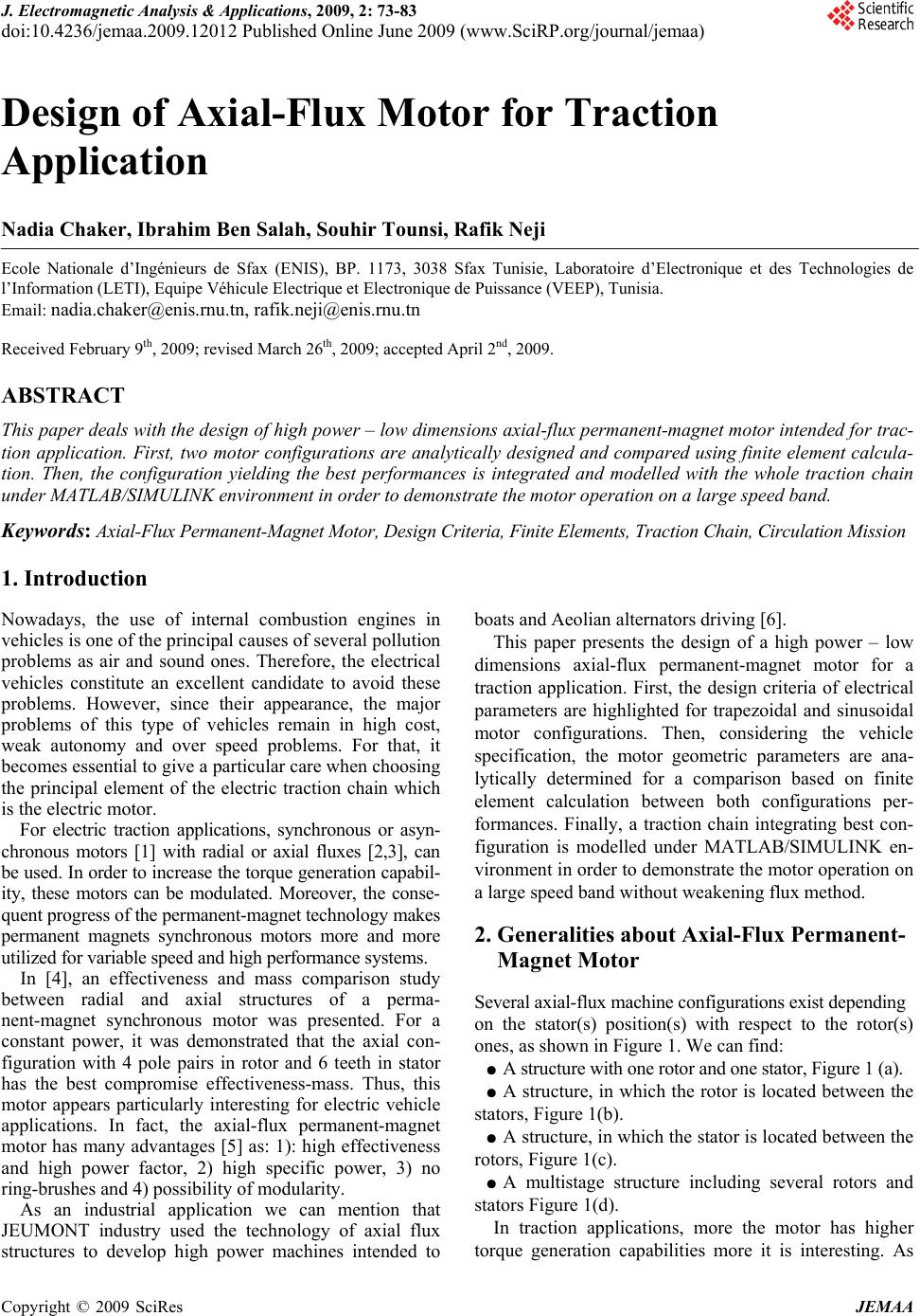J. Electromagnetic Analysis & Applications, 2009, 2: 73-83
doi:10.4236/jemaa.2009.12012 Published Online June 2009 (www.SciRP.org/journal/jemaa)
1
Design of Axial-Flux Motor for Traction
Application
Nadia Chaker, Ibrahim Ben Salah, Souhir Tounsi, Rafik Neji
Ecole Nationale d’Ingénieurs de Sfax (ENIS), BP. 1173, 3038 Sfax Tunisie, Laboratoire d’Electronique et des Technologies de
l’Information (LETI), Equipe Véhicule Electrique et Electronique de Puissance (VEEP), Tunisia.
Received February 9th, 2009; revised March 26th, 2009; accepted April 2nd, 2009.
ABSTRACT
This paper deals with the design of high power – low dimensions axial-flux permanent-magnet motor intended for trac-
tion application. First, two motor configurations are analytically designed and compared using finite element calcula-
tion. Then, the configuration yielding the best performances is integrated and modelled with the whole traction chain
under MATLAB/SIMULINK environment in order to demonstrate the motor operation on a large speed band.
Keywords: Axial-Flux Permanent-Magnet Motor, Design Criteria, Finite Elements, Traction Chain, Circulation Mission
1. Introduction
Nowadays, the use of internal combustion engines in
vehicles is one of the principal causes of several pollution
problems as air and sound ones. Therefore, the electrical
vehicles constitute an excellent candidate to avoid these
problems. However, since their appearance, the major
problems of this type of vehicles remain in high cost,
weak autonomy and over speed problems. For that, it
becomes essential to give a particular care when choosing
the principal element of the electric traction chain which
is the electric motor.
For electric traction applications, synchronous or asyn-
chronous motors [1] with radial or axial fluxes [2,3], can
be used. In order to increase the torque generation capabil-
ity, these motors can be modulated. Moreover, the conse-
quent progress of the permanent-magnet technology makes
permanent magnets synchronous motors more and more
utilized for variable speed and high performance systems.
In [4], an effectiveness and mass comparison study
between radial and axial structures of a perma-
nent-magnet synchronous motor was presented. For a
constant power, it was demonstrated that the axial con-
figuration with 4 pole pairs in rotor and 6 teeth in stator
has the best compromise effectiveness-mass. Thus, this
motor appears particularly interesting for electric vehicle
applications. In fact, the axial-flux permanent-magnet
motor has many advantages [5] as: 1): high effectiveness
and high power factor, 2) high specific power, 3) no
ring-brushes and 4) possibility of modularity.
As an industrial application we can mention that
JEUMONT industry used the technology of axial flux
structures to develop high power machines intended to
boats and Aeolian alternators driving [6].
This paper presents the design of a high power – low
dimensions axial-flux permanent-magnet motor for a
traction application. First, the design criteria of electrical
parameters are highlighted for trapezoidal and sinusoidal
motor configurations. Then, considering the vehicle
specification, the motor geometric parameters are ana-
lytically determined for a comparison based on finite
element calculation between both configurations per-
formances. Finally, a traction chain integrating best con-
figuration is modelled under MATLAB/SIMULINK en-
vironment in order to demonstrate the motor operation on
a large speed band without weakening flux method.
2. Generalities about Axial-Flux Permanent-
Magnet Motor
Several axial-flux machine configurations exist depending
on the stator(s) position(s) with respect to the rotor(s)
ones, as shown in Figure 1. We can find:
● A structure with one rotor and one stator, Figure 1 (a).
● A structure, in which the rotor is located between the
stators, Figure 1(b).
● A structure, in which the stator is located between the
rotors, Figure 1(c).
● A multistage structure including several rotors and
stators Figure 1(d).
In traction applications, more the motor has higher
torque generation capabilities more it is interesting. As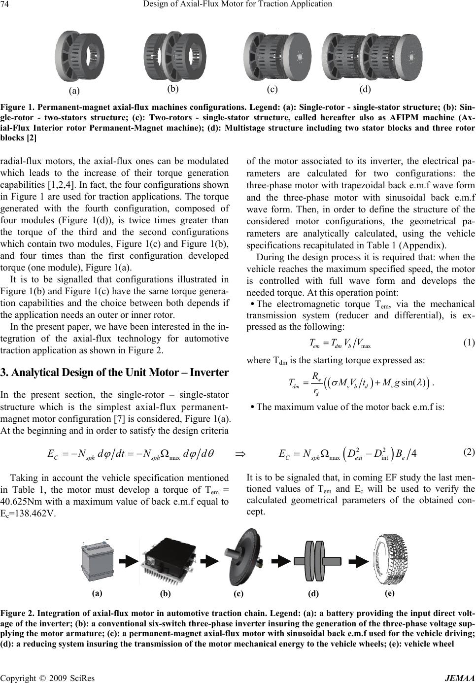

Design of Axial-Flux Motor for Traction Application 74
(b) (c) (d)
(a)
Figure 1. Permanent-magnet axial-flux machines configurations. Legend: (a): Single-rotor - single-stator structure; (b): Sin-
gle-rotor - two-stators structure; (c): Two-rotors - single-stator structure, called hereafter also as AFIPM machine (Ax-
ial-Flux Interior rotor Permanent-Magnet machine); (d): Multistage structure including two stator blocks and three rotor
blocks [2]
radial-flux motors, the axial-flux ones can be modulated
which leads to the increase of their torque generation
capabilities [1,2,4]. In fact, the four configurations shown
in Figure 1 are used for traction applications. The torque
generated with the fourth configuration, composed of
four modules (Figure 1(d)), is twice times greater than
the torque of the third and the second configurations
which contain two modules, Figure 1(c) and Figure 1(b),
and four times than the first configuration developed
torque (one module), Figure 1(a).
It is to be signalled that configurations illustrated in
Figure 1(b) and Figure 1(c) have the same torque genera-
tion capabilities and the choice between both depends if
the application needs an outer or inner rotor.
In the present paper, we have been interested in the in-
tegration of the axial-flux technology for automotive
traction application as shown in Figure 2.
3. Analytical Design of the Unit Motor – Inverter
In the present section, the single-rotor – single-stator
structure which is the simplest axial-flux permanent-
magnet motor configuration [7] is considered, Figure 1(a).
At the beginning and in order to satisfy the design criteria
of the motor associated to its inverter, the electrical pa-
rameters are calculated for two configurations: the
three-phase motor with trapezoidal back e.m.f wave form
and the three-phase motor with sinusoidal back e.m.f
wave form. Then, in order to define the structure of the
considered motor configurations, the geometrical pa-
rameters are analytically calculated, using the vehicle
specifications recapitulated in Table 1 (Appendix).
During the design process it is required that: when the
vehicle reaches the maximum specified speed, the motor
is controlled with full wave form and develops the
needed torque. At this operation point:
● The electromagnetic torque Tem, via the mechanical
transmission system (reducer and differential), is ex-
pressed as the following:
maxemdm b
TTVV

(1)
where Tdm is the starting torque expressed as:
 
sin( )
w
dmv bdv
d
R
TMVtMg
r

 .
● The maximum value of the motor back e.m.f is:


22
maxmaxint 4 CsphsphCsphexte
ENddtN ddENDDB    (2)
Taking in account the vehicle specification mentioned
in Table 1, the motor must develop a torque of Tem =
40.625Nm with a maximum value of back e.m.f equal to
Ec=138.462V.
It is to be signaled that, in coming EF study the last men-
tioned values of Tem and Ec will be used to verify the
calculated geometrical parameters of the obtained con-
cept.
(e)
(a) (b) (c) (d)
Figure 2. Integration of axial-flux motor in automotive traction chain. Legend: (a): a battery providing the input direct volt-
age of the inverter; (b): a conventional six-switch three-phase inverter insuring the generation of the three-phase voltage sup-
plying the motor armature; (c): a permanent-magnet axial-flux motor with sinusoidal back e.m.f used for the vehicle driving;
(d): a reducing system insuring the transmission of the motor mechanical energy to the vehicle wheels; (e): vehicle wheel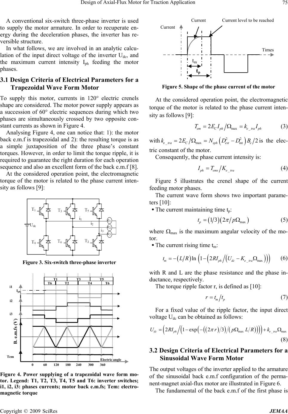

Design of Axial-Flux Motor for Traction Application 75
A conventional six-switch three-phase inverter is used
to supply the motor armature. In order to recuperate en-
ergy during the deceleration phases, the inverter has re-
versible structure.
In what follows, we are involved in an analytic calcu-
lation of the input direct voltage of the inverter Udc, and
the maximum current intensity Iph feeding the motor
phases.
3.1 Design Criteria of Electrical Parameters for a
Trapezoidal Wave Form Motor
To supply this motor, currents in 120° electric crenels
shape are considered. The motor power supply appears as
a succession of 60° electric sequences during which two
phases are simultaneously crossed by two opposite con-
stant currents as shown in Figure 4.
Analysing Figure 4, one can notice that: 1): the motor
back e.m.f is trapezoidal and 2): the resulting torque is as
a simple juxtaposition of the three phase’s constant
torques. However, in order to limit the torque ripple, it is
required to guarantee the right duration for each operation
sequence and also an excellent form of the back e.m.f [8].
At the considered operation point, the electromagnetic
torque of the motor is related to the phase current inten-
sity as follows [9]:
Figure 3. Six-switch three-phase inverter
Figure 4. Power supplying of a trapezoidal wave form mo-
tor. Legend: T1, T2, T3, T4, T5 and T6: inverter switches;
i1, i2, i3: phases currents; motor back e.m.fs; Tem: electro-
magnetic torque
Current Current level to be reached
Current
Figure 5. Shape of the phase current of the motor
At the considered operation point, the electromagnetic
torque of the motor is related to the phase current inten-
sity as follows [9]:
max _
2
emC phe tra ph
TEI kI

 (3)
with

22
_max int
22
etraCsph exte
kE NDDBis the elec-
tric constant of the motor.
Consequently, the phase current intensity is:
_
p
hemsetra
ITK

(4)
Figure 5 illustrates the crenel shape of the current
feeding motor phases.
The current wave form shows two important parame-
ters [10]:
● The current maintaining time tp:


max
13 2
p
tp  

(5)
where max is the maximum angular velocity of the mo-
tor.
● The current rising time tm:






_max
ln 12
mphdce
tLR RIUK 
tra
(6)
with R and L are the phase resistance and the phase in-
ductance, respectively.
The torque ripple factor r, is defined as [10]:
mp
rtt

(7)
For a fixed value of the ripple factor, the input direct
voltage Udc can be obtained as follows:
  






max_ max
21exp23
dcphe tra
URIr pLRk 

 
(8)
3.2 Design Criteria of Electrical Parameters for a
Sinusoidal Wave Form Motor
The output voltages of the inverter applied to the armature
of the sinusoidal back e.m.f configuration of the perma-
nent-magnet axial-flux motor are illustrated in Figure 6.
The fundamental of the back e.m.f of the first phase is
Tem
0 60 120 180240 300 360
i1
i2
i3
Iph
B. e.m.fs (V)
Electric angle
T1 T3 T5
T2 T4 T6 T6
tm
tp
Times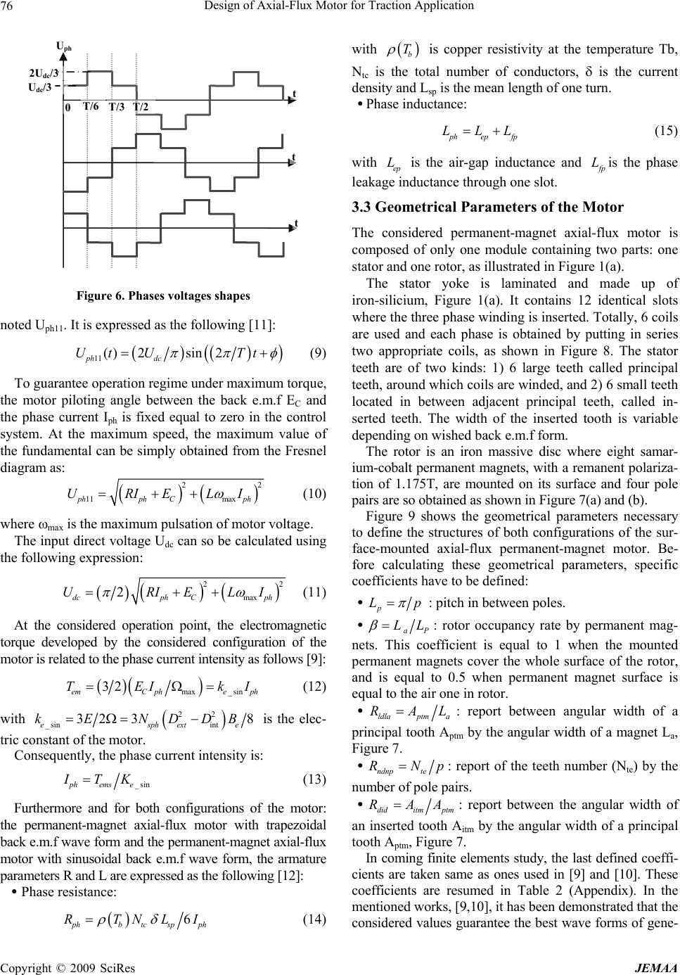

Design of Axial-Flux Motor for Traction Application 76
Figure 6. Phases voltages shapes
noted Uph11. It is expressed as the following [11]:


11 ()2sin 2 ph dc
Ut UTt



 (9)
To guarantee operation regime under maximum torque,
the motor piloting angle between the back e.m.f EC and
the phase current Iph is fixed equal to zero in the control
system. At the maximum speed, the maximum value of
the fundamental can be simply obtained from the Fresnel
diagram as:

2
11 maxphph Cph
URIELI   2 (10)
where max is the maximum pulsation of motor voltage.
The input direct voltage Udc can so be calculated using
the following expression:


2
max
2
dcph Cph
URIEL  
2
I (11)
At the considered operation point, the electromagnetic
torque developed by the considered configuration of the
motor is related to the phase current intensity as follows [9]:
 
max_ sin
32
emC pheph
TEI kI (12)
with

22
_ sinint
32 38
esphext
kE NDDB e is the elec-
tric constant of the motor.
Consequently, the phase current intensity is:
_sinphems e
ITK (13)
Furthermore and for both configurations of the motor:
the permanent-magnet axial-flux motor with trapezoidal
back e.m.f wave form and the permanent-magnet axial-flux
motor with sinusoidal back e.m.f wave form, the armature
parameters R and L are expressed as the following [12]:
● Phase resistance:

6
p
hbtcsp
RTNLI  
with


b
T  is copper resistivity at the temperature Tb,
Ntc is the total number of conductors,  is the current
density and Lsp is the mean length of one turn.
U
p
h
2Udc/3
Udc/3 t
● Phase inductance:
T/6
ph
(14)
p
hepf
LLL
p
(15)
with is the air-gap inductance and is the phase
leakage inductance through one slot.
ep
Lfp L
3.3 Geometrical Parameters of the Motor
The considered permanent-magnet axial-flux motor is
composed of only one module containing two parts: one
stator and one rotor, as illustrated in Figure 1(a).
The stator yoke is laminated and made up of
iron-silicium, Figure 1(a). It contains 12 identical slots
where the three phase winding is inserted. Totally, 6 coils
are used and each phase is obtained by putting in series
two appropriate coils, as shown in Figure 8. The stator
teeth are of two kinds: 1) 6 large teeth called principal
teeth, around which coils are winded, and 2) 6 small teeth
located in between adjacent principal teeth, called in-
serted teeth. The width of the inserted tooth is variable
depending on wished back e.m.f form.
The rotor is an iron massive disc where eight samar-
ium-cobalt permanent magnets, with a remanent polariza-
tion of 1.175T, are mounted on its surface and four pole
pairs are so obtained as shown in Figure 7(a) and (b).
Figure 9 shows the geometrical parameters necessary
to define the structures of both configurations of the sur-
face-mounted axial-flux permanent-magnet motor. Be-
fore calculating these geometrical parameters, specific
coefficients have to be defined:
● p
Lp

 : pitch in between poles.
● aP
LL


: rotor occupancy rate by permanent mag-
nets. This coefficient is equal to 1 when the mounted
permanent magnets cover the whole surface of the rotor,
and is equal to 0.5 when permanent magnet surface is
equal to the air one in rotor.
● ldlaptm a
RAL

: report between angular width of a
principal tooth Aptm by the angular width of a magnet La,
Figure 7.
● ndnp te
RNp

: report of the teeth number (Nte) by the
number of pole pairs.
● diditm ptm
RAA

: report between the angular width of
an inserted tooth Aitm by the angular width of a principal
tooth Aptm, Figure 7.
In coming finite elements study, the last defined coeffi-
cients are taken same as ones used in [9] and [10]. These
coefficients are resumed in Table 2 (Appendix). In the
mentioned works, [9,10], it has been demonstrated that the
considered values guarantee the best wave forms of gene-
0 T/3 T/2
t
t

Design of Axial-Flux Motor for Traction Application 77
(a) Trapezoidal back e.m.f configuration
(b) Sinusoidal back e.m.f configuration
Figure 7. Structures of both configurations of the perma-
nent-magnet axial-flux motor
Figure 8. Cylindrical cut plan of the stator of the axial-flux
motor
Figure 9. Geometrical parameters of the permanent-magnet
axial-flux motor. Legend: Hr: rotor disc thickness; Hpm:
permanent magnet height; Hth: slot height; Hy: stator yoke
thickness; e: air-gap thickness; Ls: slot width
rated fluxes and discard leakage fluxes between perma-
nent magnets, for trapezoidal and sinusoidal motors.
Referring to [12], the motor geometrical parameters
are calculated by integrating the mentioned coefficient in
trigonometric formulas. The obtained geometrical pa-
rameters for both motor configurations are recapitulated
in Table 2 (Appendix).
4. Finite Elements Study
In axial-flux motor, the magnetic phenomena are sym-
metrical according to the motor radial direction. Thus, the
finite elements study of the two motor configurations can
be simplified from 3D to 2D finite elements study which
is simpler and more speed from the point of view of cal-
culation time. The used software is MAXWELL 2D [13].
Figure 10 illustrates the finite elements study domain
of the trapezoidal configuration of the axial-flux motor.
In order to validate the analytical calculated parameters,
this study is intended to the computation of the generated
fluxes in the motor air-gap which yields the back e.m.fs
and the developed torque at load operation point. In the
first step, the geometrical parameters analytically calcu-
lated in Subsection 2.3 are used to define the geometry
used in the finite elements program. Then, in a second
step and for different values of the rotor position, two
different finite elements calculations are processed:
● An investigation of the effect of only the permanent
magnets: the machine is working as a generator at
no-load operation regime. The fluxes wave forms due to
the permanent magnets effect are so carried out. Conse-
quently, motor back e.m.fs wave forms and amplitudes
are deduced which characterise the electric/mechanic
power transfer.
1’
● A computation under load operation point: the cur-
rent feeding the motor armature is in phase with the back
e.m.f obtained through the previous study. The so gener-
ated flux is used to find out the machine torque.
Figure 11 shows the flux lines through the magnetic
circuit of the sinusoidal wave form configuration of the
axial-flux motor due to the effect of only the permanent
magnets and Figure 12 shows the flux lines through the
magnetic circuit of the sinusoidal wave form configura-
tion of the axial-flux motor under load operation.
Analyzing these figures, one can notice that leakage
fluxes between permanent magnets do not exist and all
generated fluxes are useful.
4.1 Finite Elements Study at Generation Mode
For both configurations of the axial-flux motor, the con-
sidered operation point corresponds to the maximum
speed of the vehicle (80km/h) which means an angular
velocity equal to 341.88rad/s. For trapezoidal configura-
2 2 3’ 3’ 1 1 2’ 2’ 3 31’
North
magnet
Stator yoke
Rotor disc
South magnet
Principal tooth
Hr
Inserted tooth
Slot
Hy
Hth
e
Hpm
Ls

Design of Axial-Flux Motor for Traction Application 78
Figure 10. Cylindrical cut plan of the trapezoidal wave form motor
Figure 11. Flux lines through the magnetic circuit of the sinusoidal wave form configuration of the axial-flux motor due to the
effect of only the permanent magnets
Figure 12. Flux lines through the magnetic circuit of the sinusoidal wave form configuration of the axial-flux motor under
load operation
-0,010
-0,008
-0,006
-0,004
-0,002
0,000
0,002
0,004
0,006
0,008
0,010
0 10203040506070809
Angle (°)
Flux (Wb)
0
Flux1_no-load Flux2_no-load Flux3_no-load
-0,008
-0,006
-0,004
-0,002
0,000
0,002
0,004
0,006
0,008
0 10203040506070809
Angle (°)
Flux (Wb)
0
Flux1_no-load Flux2_no-load Flux3_no-load
(a) Trapeze case (b) Sine case
Figure 13. Fluxes generated in the air-gap of the machine for a generation regime at no-load operation and for a vehicle speed
of 80km/h
tion and sinusoidal one, the wave form of generated
fluxes in the air-gap are illustrated respectively in Figure
For each motor phase, the back e.m.f can be obtained
considering a perfect magnetic circuit and using the fol-
lowing expression: 13(a) and (b) where rotor position is varied from 0° to 90°.





Csph phsphphsphph
etNd dtNddtd dNd d





   (16)
with

is the rotor position and
p
h

is the flux of the
considered phase.
The differential ph dd

 can be obtained by a lin-
earization between two consecutive positions and the
back e.m.f is so expressed as:



112
() ()
Csph phph
eN 12





  (17)
Figure 14 shows the wave form of the obtained back
e.m.fs for both axial-flux motor configurations.
Analyzing those figures one can remark that in the case
of the trapezoidal configuration of the motor the gener-
ated back e.m.fs are perfectly trapezoidal and in the case
of the sinusoidal motor configuration the generated back
e.m.fs are also perfectly sinusoidal.
4.2 Finite Elements Study under Load Operation
In this section, the motor is considered under load opera-
tion regime. The motor armature is supplied by three
currents in phase with the back e.m.fs obtained at the
no-load operation of the generation regime. As illustrated
in Figure 15(a) and (b), crenel shape currents with a maxi-
mum intensity Iph_trapeze = 50.154A are used for the trape-
zoidal configuration, and sinusoidal shape currents with a

Design of Axial-Flux Motor for Traction Application 79
-200
-150
-100
-50
0
50
100
150
200
0 10203040506070809
Angle (°)
Back e.m.f (V)
0
Back e.m.f 1_no-loadBack e.m.f 2_no-loadBack e.m.f 3_no-load
-200
-150
-100
-50
0
50
100
150
200
0 10203040506070809
Angle (°)
Back e.m.f (V)
0
Back e.m.f 1_no-loadBack e.m.f 2_no-loadBack e.m.f 3_no-load
(a) Trapeze case (b) Sine case
Figure 14. Wave form of the generated back e.m.f for a generation regime at no-load operation and for a vehicle speed of 80km/h
maximum intensity Iph_sine = 66.872A are used for the
sinusoidal configuration.
Figure 15(c) and Figure 15(d) illustrate the wave form
of obtained fluxes in the motor air-gap for the maximum
vehicle speed (80 km/h), and different rotor positions
varying from 0° to 90°, respectively for trapezoidal and
sinusoidal motors. Analysing these figures, one can notice
the appearance of flux distortion at the load operation re-
gime in respect with the no-load operation one. This dis-
tortion is essentially due to the magnetic armature reaction.
Considering Equation (16) and for a perfect magnet
circuit, the back e.m.f of the motor can be calculated and
illustrated as shown in Figure 15(e) and (f) for trapezoi-
dal and sinusoidal configurations, respectively. Referring
to the aforementioned figures, one can remark the fol-
lowing: 1): for both configurations the analytical maxi-
mum value of the back e.m.f Ec = 138.462V is reached,
2): the sinusoidal configuration generates a sinusoidal
back e.m.f without peaks which yields a torque wave
form with no peaks, Figure 15(h). However, the trape-
zoidal configuration generates a trapezoidal distorted
back e.m.f containing several peaks giving a torque wave
form with several peaks too, Figure 15(g).
Referring to Figure 15(g) and (h), both motors are able
to develop the requested torque. The ripple figuring in the
torques wave forms is due essentially to the motors cog-
ged structures which cause the appearance of a cogging
torque. Considering the obtained torques wave forms,
vibration problems due to the torque ripple are sharper in
the case of trapezoidal motor than in the case of the si-
nusoidal one. For that, in coming study, only the features
of the permanent-magnet axial-flux sinusoidal motor are
investigated.
5. Traction Chain Modelling
The present section is devoted to the modelling of an
axial-flux motor with sinusoidal back e.m.f wave form
associated to a six-switch three-phase inverter for traction
application. The whole traction chain is modelled in order
to investigate the motor behaviour vis-à-vis of a desired
speed sequence and of the circulation mission of the Na-
tional Institute of Research on Transports and their Secu-
rity (INRETS).
Figure 16 shows the block diagram of the adopted
control vector strategy of the motor implemented under
MATLAB/SIMULINK environment.
The synchronous permanent magnet machine can be
described in the d-q referential as follows [14]:



ddddeqq
qqqqedde
VRiLdidt Li
VRiLdidtLiK

m


 

 


(18)
with e is the electric pulsation, Ld and Lq are respec-
tively direct in squaring inductances.
The direct and in squaring components of the current
can be deduced using:



ddeqqd
qqeddemq
IV LiLSR
I
VLiK LS


 

R

 


(19)
with S is Laplace operator.
The developed electromagnetic torque is so expressed
[15]:



 
32 12
eme qdqdq
TKIpLLII (20)
Considering the fundamental dynamic law describing
the vehicle motion, the torque needed on wheels is:
wbraerog vwrvw
TTTTMRdVdtTMRdVdt




(21)
with Tbr is the torque due to bearing resistance force, Taero
is the torque due to aerodynamic load, Tg is the torque
due to gravity forces,  a coefficient related to the inertia

Design of Axial-Flux Motor for Traction Application 80
Trapezoidal Sinusoidal
-60
-40
-20
0
20
40
60
0 10203040506070809
Angle (°)
Current (A)
0
I1 I2 I3
(a) Three phase current
-80
-60
-40
-20
0
20
40
60
80
0 10203040506070809
Angle (°)
Current (A)
0
I1 I2I3
(b) Three phase current
-0,010
-0,008
-0,006
-0,004
-0,002
0,000
0,002
0,004
0,006
0,008
0,010
0 10203040506070809
Angle (°)
Flux (Wb)
0
Flux1_load Flux2_loadFlux3_load
(c) Air-gap fluxes
-0,008
-0,006
-0,004
-0,002
0,000
0,002
0,004
0,006
0,008
0 10203040506070809
Angle (°)
Flux (Wb)
0
Flux1_load Flux2_loadFlux3_load
(d) Air-gap fluxes
-250
-200
-150
-100
-50
0
50
100
150
200
250
0 10203040506070809
Angle (°)
Back e.m.f (V)
0
Back e.m.f 1_loadBack e.m.f 2_loadBack e.m.f 3_load
(e) Back e.m.fs
-200
-150
-100
-50
0
50
100
150
200
0 10203040506070809
Angle (°)
Back e.m.f (V)
0
Back e.m.f 1_load Back e.m.f 2_load Back e.m.f 3_load
(f) Back e.m.fs
0
10
20
30
40
50
60
70
0 10203040506070809
Angle (°)
Torque (Nm)
0
T_analytic T_load
(g) Electromagnetic torque
0
10
20
30
40
50
0 20406080
Angle (°)
Torque (Nm)
100
T_analytic T_load
(h) Electromagnetic torque
Figure 15. Load operation of trapezoidal and sinusoidal motor configurations

Design of Axial-Flux Motor for Traction Application 81
3
C3
2
C2
1
C1
triangular
signal
Sine Wave2
Sine Wave1
Sine Wave
Re lay 2
Re lay 1
Relay
C1
C2
C3
Figure 16. Block diagram of the vector control strategy of the axial-flux motor Figure 16. Block diagram of the vector control strategy of the axial-flux motor
of turning parts (wheels, driving shaft and gearing system)
and Tr is the resistive torque.
of turning parts (wheels, driving shaft and gearing system)
and Tr is the resistive torque.
The control strategy block diagram, shown in Figure
16, presents two regulation loops: the first loop is used
for speed regulation and the second one for current regu-
lation. The control vector strategy operates with only the
in squaring component of the current. For that the direct
current is cancelled and its reference value is fixed to
zero. Consequently, referring to Equation (20), the de-
veloped electromagnetic torque is expressed as:
The control strategy block diagram, shown in Figure
16, presents two regulation loops: the first loop is used
for speed regulation and the second one for current regu-
lation. The control vector strategy operates with only the
in squaring component of the current. For that the direct
current is cancelled and its reference value is fixed to
zero. Consequently, referring to Equation (20), the de-
veloped electromagnetic torque is expressed as:

32
eme q
TKI (22)
The Inverter switches are driven using PWM control
signals and the three voltages provided to supply the mo-
tor armature are:





112
221
332
32
32
32
ph dc
ph dc
ph dc
UU CCC
UU CCC
UU CCC








3
3
1



(23)
with Uph1, Uph2, Uph3 are the three phase voltage provided
by the inverter, and C1, C2, C3 are the command constants
for the inverter high transistors T1, T3 and T5, respectively.
The constants C1, C2 and C3 are generated using a
PWM generation block, Figure 17, based on the com-
parison between a triangular signal which frequency is
equal to the desired commutation frequency of the in-
verter switches and a sinusoidal one which pulsation
gives the desired motor speed. A transistor switched on
corresponds to C = 1, and a transistor switched off corre-
sponds to C = 0.
At vehicle maximum speed (80km) and for the geo-
metrical parameters analytically calculated and validated
by the finite elements study, the direct voltage applied to
the inverter Udc, the motor resistance R, the direct induc-
tance of the motor Ld, the in squaring inductance of the
motor Lq and the electric constant of the motor Ke are
analytically determined, Table 3 (Appendix). For the ob-
tained values and for a switching frequency fc = 3.3kHz,
the inverter provides three chopped and equilibrated
voltages to supply motor armature, Figure 18.
5.1 Simulation Results
5.1.1 Speed Sequence
The desired speed sequence, Figure 19, requires three
speed levels. Considering the parameters given by Table 3,
Figure 17. Generation of the inverter command constants
PI
0
PI
PI
dq 2 abc
PWM generation
Inverter
Iq ref C1
VqVa
+
PMSM
abc 2 dq
-
+
-
+
-
-
-

m
IdVd
C2
Vb
C3
Vc

Design of Axial-Flux Motor for Traction Application 82
00.001 0.002 0.003 0.004 0.005 0.006 0.007 0.008 0.009 0.01
-200
-150
-100
-50
0
50
100
150
200
Time (s)
Chopped voltage (V)
Figure 18. Motor phase chopped voltage provided at the
output of the inverter
the motor speed carried out using the traction elaborated
traction chain model is illustrated in Figure 19. Analyzing
this figure, one can notice that the vehicle speed reaches
the wanted value in a relatively weak time.
5.1.2 Circulation Mission
To validate the use of a motor for traction application, the
INRETS tests the behaviour of such motor using the
speed instruction illustrated in Figure 20(a). Such speed
instruction is called circulation mission. It consists of a
normalised trial for vehicle motor tested for long dis-
tances and variable speed under hard constraints.
In the last section, the designed motor was able to fol-
low a desired speed instruction. For the present study, let
us consider the INRETS circulation mission and investi-
gate the motor behaviour.
Figure 20(b) shows that the electric vehicle speed fol-
lows to the required circulation mission with a little delay
as found in Subsection 5.1.1.
6. Conclusions
The present paper was devoted to the design of high
power – low dimensions axial-flux permanent-magnet
motor for electric vehicles. In a first step, the electrical
and the geometrical parameters of the motor integrated in
the whole traction chain was analytically calculated con-
sidering the vehicle specifications. Then in a second step,
we have been interested in a finite elements study in or-
der to validate and complete the analytical obtained re-
sults. It has been found, that the built analytical model
provides accurate values of electrical and geometrical
motor parameters. Furthermore, a comparison between
the electromagnetic torque obtained by the trapezoidal
configuration and one developed by the sinusoidal con-
figuration was made using the finite elements study. The
high ripple noticed in the wave form of trapezoidal mo-
tor’s torque leads to discard this configuration and em-
phasize the choice of sinusoidal configuration for traction
applications. Finally, the designed sinusoidal motor be-
haviour was investigated considering firstly a desired
0 2 46 81012 14 16 18 20
0
10
20
30
40
50
60
70
80
Time (s)
Vehicle speed (Km/h)
Desired speed sequence
Electric vehicle response
Figure 19. Desired speed sequence and motor speed carried out using the developed traction chain model

Design of Axial-Flux Motor for Traction Application 83
0100 200 300 400 500 600700 800 900 1000
0
10
20
30
40
50
60
70
80
Time (s)
Vehicle Speed (Km/h)
0100 200 300 400 500 600 700 800 900 1000
0
10
20
30
40
50
60
70
80
Time (s)
Vehicle speed (Km/h)
(a) INRETS circulation mission (b) Electric vehicle response
Figure 20. INRETS circulation mission and electric vehicle response
speed instruction and next the INRETS circulation mis-
sion. For that, we have been involved in the modelling
and implementation under matlab/simulink environment
of such motor associated to six-switch three-phase in-
verter and integrated in the whole traction chain. For both
tests, the motor was able to follow and to provide the
requested features which make the sinusoidal axial-flux
permanent-magnet motors serious competitors of con-
ventional radial-flux permanent-magnet motors for
automotive traction applications.
Appendix
Table 1. Motor specification
Parameter symbol value unit
Vehicle mass Mv 800
kg
Wheel ray Rw 0.26
m
Basic velocity Vb 30
km/h
Maximum speed of the vehicle Vmax 80
km/h
Pole pair number p 4
Stating time td 4
s
Coefficient related to the inertia if the turning parts  1
Switched frequency fc 3.33
kHz
Reduction report rd 4
Gravity g 9.81 N/kg
External diameter Dext 350 mm
Internal diameter Dint 150 mm
Table 2. Motor dimensioning
Designation Symbol Trapeze Sine
Report of the teeth number by the number of pole pairs Rndnp 1.5 1.5
Rotor occupancy rate by permanent magnets β 1 2/3
Report between angular width of a principal tooth by the angular width of a magnet Rldla 1 1
Report between the angular widths of an inserted tooth by the angular width of a principal toot. Rdid 0.2 0.2
Rotor disc thickness Hr 83.357 mm 55.611 mm
Permanent magnets height Hpm 6.873 mm 6.873 mm
Slots height Hth 69.671 mm 17.214 mm
Stator yoke thickness Hy 98.176 mm 65.498 mm
Slots mean angular width Asm 3° 12°
Slots width Ls 6.545 mm 26.132mm
Magnet mean angular width La 45° 30°
Principal tooth mean angular width Aptm 45° 30°
Inserted tooth mean angular width Aitm 9° 6°
Air-gap thickness e 2 mm 2 mm

Design of Axial-Flux Motor for Traction Application 84
Table 3. Electric parameters used for the simulation of the traction chain model
Parameter symbol value unit
Direct voltage Udc 291
V
Drag coefficient Cx 0.55
Frontal surface Sf 1.8
m²
Coefficient to bearing pneumatic resistance fr 0.01
Electric constant Ke 0.3
Phase resistance Rph 0.007
Ω
Direct inductance Ld 0.157
mH
In squaring inductance Lq 0.157
mH
REFERENCES
[1] Y. Amara, “Contribution à la conception et à la
commande des machines synchrones à double excitation,
Application au véhicule hybride,” Thèse de doctorat,
université, PARIS VI, 2001.
[2] A. Parviainen, “Design of axial-flux permanent-magnet
low-speed machines and performance comparison be-
tween radial-flux and axial-flux machines,” thesis of doc-
torate, Lappeeranta University of Technology, Lappeer-
anta, Finland, 2005.
[3] A. Parviainen, M. Niemelä, J. Pyrhönen, J. Mantere,
“Performance comparison between low-speed axial-flux
and radial flux permanent-magnet machines including
mechanical constraints,” Electric Machines and Drives,
IEEE International Conference, pp. 1695–1702, 2005.
[4] S. Tounsi, “Modélisation et optimisation de la motori-
sation et de l’autonomie d’un véhicule électrique,” Thèse
de doctorat en Génie Electrique, Ecole Nationale
d’Ingénieurs de Sfax-Tunisie, 2006.
[5] B. Multon and J. Bonal, “Les entraînements électro-
magnétiques directs: Diversité, contraintes et solutions, La
conversion électromécanique directe,” - ENS Cachan –
SEE, 1999.
[6] P. Kurronen, “Torque vibration model of axial-flux sur-
face-mounted permanent magnet synchronous machine,”
Dissertation, Lappeenranta University of Technology,
Finland, 2003.
[7] B. Tounsi, “Etude comparative de groupes électrogènes
embarqués à large gamme de vitesse variable associant
machines à aimants permanents et conversion statique,”
Thèse de Doctorat, INP Toulouse, 2006.
[8] S. Tounsi, R. Neji, and F. Sellami, “Contribution à la
conception d’un Actionneur à Aimants Permanents pour
Véhicules Electriques en vue d’Optimiser l’Autonomie,”
Revue Internationale de Génie Electrique, RIGE, Vol. 9/6,
pp. 693-718, Edition Lavoisier, 2006.
[9] C. Cavallaro, A. O. Di Tommaso, R. Miceli, A. Raciti, G.
R. Galluzzo, and M. Trapanese, “Efficiency enhancement
of permanent-magnet synchronous motor drives by online
loss minimization approaches,” IEEE Transactions on
Industrial Electronics, Vol. 52, No. 4, pp. 1153-1160,
2005.
[10] R. Neji, S. Tounsi, and F. Sellami, “Contribution to the
definition of a permanent magnet motor with reduced
production cost for the electrical vehicle propulsion,”
European Transactions on Electrical Power, ETEP, Vol.
16, No. 4, pp. 437-460, 2006.
[11] R. Neji, S. Tounsi, and F. Sellami, “Optimization and
design for a radial flux permanent magnet motor for elec-
tric vehicle,” Journal of Electrical Systems, JES, Vol. 1,
No. 4, 2005.
[12] N. Chaker, “Conception et commande d’un moteur à
aimant permanent à flux axial pour véhicule électrique,”
Mémoire de Mastère en génie électrique, Ecole Nationale
d’Ingénieurs de Sfax, Tunisie, 2006.
[13] MAXWELL® 2D (2002) Student Version; A 2D Magne-
tostatic Problem.
[14] F. Khatounian, S. Moreau, J. P. Louis, E. Monmasson, F.
Louveau, and J. M. Alexandre, “Modeling and simulation
of a hybrid dynamic system used in haptic interfaces,”
Electrimacs, Hammamet, Tunisie, 2005.
[15] G. Kayhan, A. A. Ahmed, and P. Halit, “Improving the
performance of hysteresis direct torque control of IPMSM
using active filter topology,” S¯adhan¯a, Vol. 31, Part 3,
pp. 245–258, 2006.