 Journal of Service Science and Management, 2011, 4, 66-78 doi:10.4236/jssm.2011.41010 Published Online March 2011 (http://www.SciRP.org/journal/jssm) Copyright © 2011 SciRes. JSSM Ambulance Deployment and Shift Scheduling: An Integrated Approach Hari K. Rajagopalan1, Cem Saydam2, Elizabeth Sharer1, Hubert Setzler1 1School of Business, Francis Marion University Florence, Florence, USA; 2Belk College of Business, The University of North Carolina at Charlotte, Charlotte, USA. Email: hrajagopalan@fmarion.edu Received October 14th, 2010; revised November 23rd, 2010; accepted November 27th, 2010.5 ABSTRACT Emergency medical response providers’ primary responsibility is to deploy an adequate number of ambulances in a manner that will yield the best service to a constituent population. In this paper we develop a two-stage integrated solu- tion for complex ambulance deployment and crew shift scheduling. In the first stage we develop a dynamic expected coverage model to determine the minimum number of ambulances and their locations for each time interval and solve via a tabu search. For the second stage, we develop an integer programming model which uses the solution obtained from the first stage to determine optimal crew schedules. We present computational statistics and demonstrate the effi- cacy of our two-stage solution approach using a case study. Keywords: Ambulance Location, Dynamic Relocation, Shift Scheduling, Hypercube 1. Introduction Emergency medical service (EMS) providers’ ultimate goal is that at any given moment an ambulance can reach a medical emergency within a predefined time standard. Although there is no universally accepted response time standard in the U.S. the most widely used EMS (ambu- lance) response time standard is based on National Fire Protection Association (NFPA) 1720 [1] which is 8 min- utes 59 seconds (inclusive of the 60 seconds of call han- dling time) for 90 percent of life threatening calls [2]. In order to meet the response time standard EMS adminis- trators must determine the minimum number of ambu- lances they need to deploy in order to provide the re- quired coverage consistently over the entire service area. However, demand often fluctuates both temporally and spatially. The volume of demand at 2 am in the morning is likely to be very different from the volume of demand at 9 am or 5 pm. Also, where demand originates from changes with time. During morning rush hours people tend to travel towards city center, business and industrial parks, and schools and universities. Generally this kind of population flow reverses direction during afternoon rush hours. Data analyses from various metropolitan ar- eas show significant variability in both volume and loca- tion of demand for EMS services [2,3]. Therefore, given such demand fluctuations, EMS administrators must first determine the optimal quantity and location of ambu- lances to meet, or exceed, a given time standard. Subse- quently, they develop weekly work schedules. Develop- ing optimal work schedules for ambulance crews is fur- ther complicated by variable shift lengths which typically range from ten, twelve or fourteen hours. In summary, EMS administrators make decisions from a set of com- plex choices. First, based on projected call volume for various sectors of a region, they must decide on where, and how many units to deploy, for each time interval which could be as small as an hour. Second, using the number of ambulances deployed, their locations (posts) for each time interval and the given shift lengths as in- puts, a schedule has to be developed. In this paper, a two-stage solution approach to this problem is developed. In the first stage the minimum number of ambulances is determined along with the locations where they need to be deployed and the number of redeployments to ensure coverage over each time interval. In the second stage, an integer programming model is formulated to determine the optimal shift schedule using the inputs from the first stage. This paper is organized as follows. Section 2 contains the literature review. Section 3 presents the dynamic ex- pected coverage location problem (DECL) and the solu- 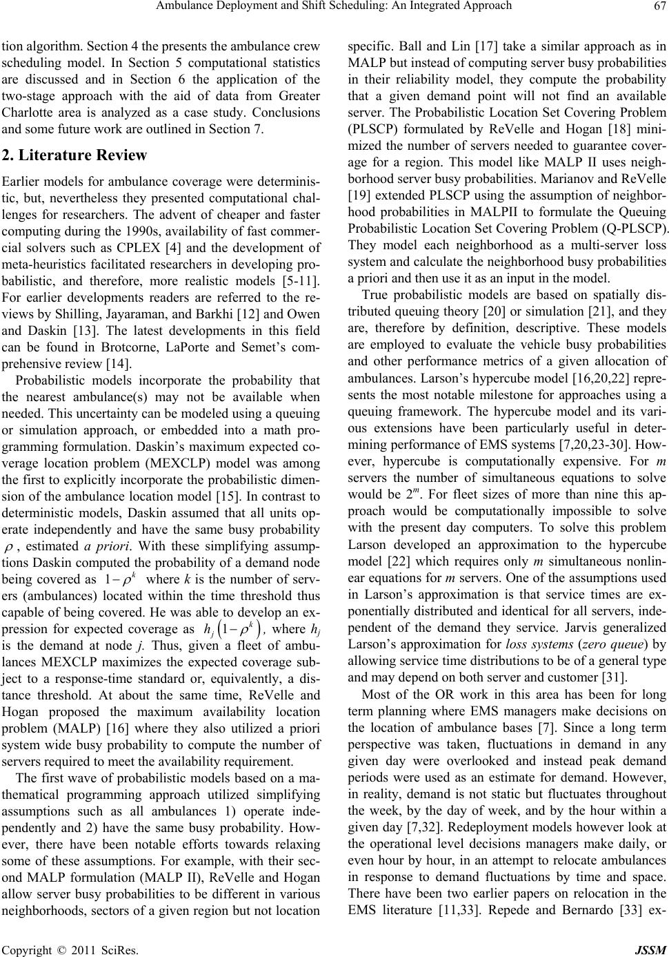 Ambulance Deployment and Shift Scheduling: An Integrated Approach 67 tion algorithm. Section 4 the presents the ambulance crew scheduling model. In Section 5 computational statistics are discussed and in Section 6 the application of the two-stage approach with the aid of data from Greater Charlotte area is analyzed as a case study. Conclusions and some future work are outlined in Section 7. 2. Literature Review Earlier models for ambulance coverage were determinis- tic, but, nevertheless they presented computational chal- lenges for researchers. The advent of cheaper and faster computing during the 1990s, availability of fast commer- cial solvers such as CPLEX [4] and the development of meta-heuristics facilitated researchers in developing pro- babilistic, and therefore, more realistic models [5-11]. For earlier developments readers are referred to the re- views by Shilling, Jayaraman, and Barkhi [12] and Owen and Daskin [13]. The latest developments in this field can be found in Brotcorne, LaPorte and Semet’s com- prehensive review [14]. Probabilistic models incorporate the probability that the nearest ambulance(s) may not be available when needed. This uncertainty can be modeled using a queuing or simulation approach, or embedded into a math pro- gramming formulation. Daskin’s maximum expected co- verage location problem (MEXCLP) model was among the first to explicitly incorporate the probabilistic dimen- sion of the ambulance location model [15]. In contrast to deterministic models, Daskin assumed that all units op- erate independently and have the same busy probability , estimated a priori. With these simplifying assump- tions Daskin computed the probability of a demand node being covered as 1k where k is the number of serv- ers (ambulances) located within the time threshold thus capable of being covered. He was able to develop an ex- pression for expected coverage as 1k j h , where hj is the demand at node j. Thus, given a fleet of ambu- lances MEXCLP maximizes the expected coverage sub- ject to a response-time standard or, equivalently, a dis- tance threshold. At about the same time, ReVelle and Hogan proposed the maximum availability location problem (MALP) [16] where they also utilized a priori system wide busy probability to compute the number of servers required to meet the availability requirement. The first wave of probabilistic models based on a ma- thematical programming approach utilized simplifying assumptions such as all ambulances 1) operate inde- pendently and 2) have the same busy probability. How- ever, there have been notable efforts towards relaxing some of these assumptions. For example, with their sec- ond MALP formulation (MALP II), ReVelle and Hogan allow server busy probabilities to be different in various neighborhoods, sectors of a given region but not location specific. Ball and Lin [17] take a similar approach as in MALP but instead of computing server busy probabilities in their reliability model, they compute the probability that a given demand point will not find an available server. The Probabilistic Location Set Covering Problem (PLSCP) formulated by ReVelle and Hogan [18] mini- mized the number of servers needed to guarantee cover- age for a region. This model like MALP II uses neigh- borhood server busy probabilities. Marianov and ReVelle [19] extended PLSCP using the assumption of neighbor- hood probabilities in MALPII to formulate the Queuing Probabilistic Location Set Covering Problem (Q-PLSCP). They model each neighborhood as a multi-server loss system and calculate the neighborhood busy probabilities a priori and then use it as an input in the model. True probabilistic models are based on spatially dis- tributed queuing theory [20] or simulation [21], and they are, therefore by definition, descriptive. These models are employed to evaluate the vehicle busy probabilities and other performance metrics of a given allocation of ambulances. Larson’s hypercube model [16,20,22] repre- sents the most notable milestone for approaches using a queuing framework. The hypercube model and its vari- ous extensions have been particularly useful in deter- mining performance of EMS systems [7,20,23-30]. How- ever, hypercube is computationally expensive. For m servers the number of simultaneous equations to solve would be 2m. For fleet sizes of more than nine this ap- proach would be computationally impossible to solve with the present day computers. To solve this problem Larson developed an approximation to the hypercube model [22] which requires only m simultaneous nonlin- ear equations for m servers. One of the assumptions used in Larson’s approximation is that service times are ex- ponentially distributed and identical for all servers, inde- pendent of the demand they service. Jarvis generalized Larson’s approximation for loss systems (zero queue) by allowing service time distributions to be of a general type and may depend on both server and customer [31]. Most of the OR work in this area has been for long term planning where EMS managers make decisions on the location of ambulance bases [7]. Since a long term perspective was taken, fluctuations in demand in any given day were overlooked and instead peak demand periods were used as an estimate for demand. However, in reality, demand is not static but fluctuates throughout the week, by the day of week, and by the hour within a given day [7,32]. Redeployment models however look at the operational level decisions managers make daily, or even hour by hour, in an attempt to relocate ambulances in response to demand fluctuations by time and space. There have been two earlier papers on relocation in the EMS literature [11,33]. Repede and Bernardo [33] ex- Copyright © 2011 SciRes. JSSM 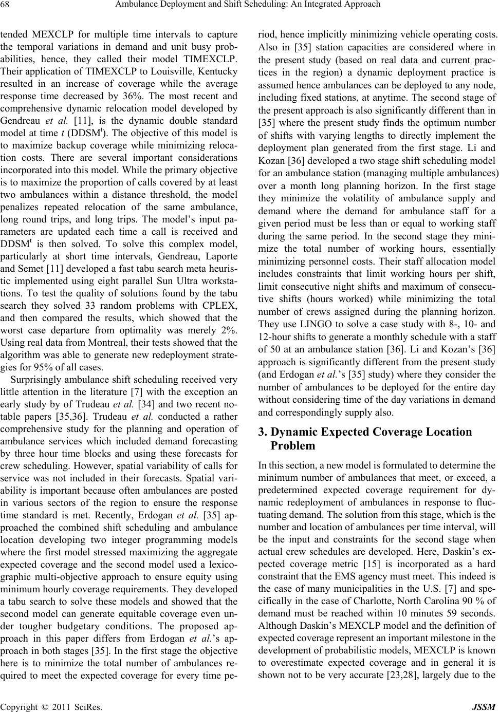 Ambulance Deployment and Shift Scheduling: An Integrated Approach 68 tended MEXCLP for multiple time intervals to capture the temporal variations in demand and unit busy prob- abilities, hence, they called their model TIMEXCLP. Their application of TIMEXCLP to Louisville, Kentucky resulted in an increase of coverage while the average response time decreased by 36%. The most recent and comprehensive dynamic relocation model developed by Gendreau et al. [11], is the dynamic double standard model at time t (DDSMt). The objective of this model is to maximize backup coverage while minimizing reloca- tion costs. There are several important considerations incorporated into this model. While the primary objective is to maximize the proportion of calls covered by at least two ambulances within a distance threshold, the model penalizes repeated relocation of the same ambulance, long round trips, and long trips. The model’s input pa- rameters are updated each time a call is received and DDSMt is then solved. To solve this complex model, particularly at short time intervals, Gendreau, Laporte and Semet [11] developed a fast tabu search meta heuris- tic implemented using eight parallel Sun Ultra worksta- tions. To test the quality of solutions found by the tabu search they solved 33 random problems with CPLEX, and then compared the results, which showed that the worst case departure from optimality was merely 2%. Using real data from Montreal, their tests showed that the algorithm was able to generate new redeployment strate- gies for 95% of all cases. Surprisingly ambulance shift scheduling received very little attention in the literature [7] with the exception an early study by of Trudeau et al. [34] and two recent no- table papers [35,36]. Trudeau et al. conducted a rather comprehensive study for the planning and operation of ambulance services which included demand forecasting by three hour time blocks and using these forecasts for crew scheduling. However, spatial variability of calls for service was not included in their forecasts. Spatial vari- ability is important because often ambulances are posted in various sectors of the region to ensure the response time standard is met. Recently, Erdogan et al. [35] ap- proached the combined shift scheduling and ambulance location developing two integer programming models where the first model stressed maximizing the aggregate expected coverage and the second model used a lexico- graphic multi-objective approach to ensure equity using minimum hourly coverage requirements. They developed a tabu search to solve these models and showed that the second model can generate equitable coverage even un- der tougher budgetary conditions. The proposed ap- proach in this paper differs from Erdogan et al.’s ap- proach in both stages [35]. In the first stage the objective here is to minimize the total number of ambulances re- quired to meet the expected coverage for every time pe- riod, hence implicitly minimizing vehicle operating costs. Also in [35] station capacities are considered where in the present study (based on real data and current prac- tices in the region) a dynamic deployment practice is assumed hence ambulances can be deployed to any node, including fixed stations, at anytime. The second stage of the present approach is also significantly different than in [35] where the present study finds the optimum number of shifts with varying lengths to directly implement the deployment plan generated from the first stage. Li and Kozan [36] developed a two stage shift scheduling model for an ambulance station (managing multiple ambulances) over a month long planning horizon. In the first stage they minimize the volatility of ambulance supply and demand where the demand for ambulance staff for a given period must be less than or equal to working staff during the same period. In the second stage they mini- mize the total number of working hours, essentially minimizing personnel costs. Their staff allocation model includes constraints that limit working hours per shift, limit consecutive night shifts and maximum of consecu- tive shifts (hours worked) while minimizing the total number of crews assigned during the planning horizon. They use LINGO to solve a case study with 8-, 10- and 12-hour shifts to generate a monthly schedule with a staff of 50 at an ambulance station [36]. Li and Kozan’s [36] approach is significantly different from the present study (and Erdogan et al.’s [35] study) where they consider the number of ambulances to be deployed for the entire day without considering time of the day variations in demand and correspondingly supply also. 3. Dynamic Expected Coverage Location Problem In this section, a new model is formulated to determine the minimum number of ambulances that meet, or exceed, a predetermined expected coverage requirement for dy- namic redeployment of ambulances in response to fluc- tuating demand. The solution from this stage, which is the number and location of ambulances per time interval, will be the input and constraints for the second stage when actual crew schedules are developed. Here, Daskin’s ex- pected coverage metric [15] is incorporated as a hard constraint that the EMS agency must meet. This indeed is the case of many municipalities in the U.S. [7] and spe- cifically in the case of Charlotte, North Carolina 90 % of demand must be reached within 10 minutes 59 seconds. Although Daskin’s MEXCLP model and the definition of expected coverage represent an important milestone in the development of probabilistic models, MEXCLP is known to overestimate expected coverage and in general it is shown not to be very accurate [23,28], largely due to the Copyright © 2011 SciRes. JSSM  Ambulance Deployment and Shift Scheduling: An Integrated Approach 69 assumptions of no server cooperation and same system wide busy probability. This model is inspired by Maria- nov and ReVelle’s Q-PSCLP [37] where they utilize neighborhood based busy probabilities instead of a sys- tem-wide busy probability. However, these probabilities are still computed a priori. This model is extended by computing server and location specific busy probabilities using Jarvis’ hypercube approximation [31]. This permits the expected coverage resulting from a given deployment to be computed more accurately. This model also incor- porates the dynamic nature of the problem where ambu- lance fleet size and locations must be determined in re- sponse to fluctuating demand throughout the day. The dynamic expected coverage location (DECL) model is formulated to deploy minimum number of am- bulances to guarantee a system wide coverage under dy- namic demand conditions. Let, t be the index of time intervals from 1 to T, hj,t be the fraction of demand at node j at time interval t, n be the number of nodes in the system, ct be the minimum expected coverage require- ment at time t, ρk,t be the busy probability of the kth pre- ferred server for a given demand node at time interval t, ρt be the average system busy probability at time interval t, m be the total number of servers available for deploy- ment and set Nj is the set of all servers that can cover node j. To be able to compute server specific busy prob- abilities, each server located at a given node must be identified. Hence, the main decision variable is defined as follows: ,, 1 if server is located at node at time 0 otherwise jkt kj x t kt lt . Conversely, the servers who cover node j are tracked with the following decision variable: ,, 1 if node is covered by server at time 0 otherwise jkt j y In developing expressions for the expected coverage requirement constraint, location-specific server busy pro- babilities, ρk, are computed using Jarvis’ hypercube ap- proximation algorithm and the correction factor (Q fac- tor). Note that the Q factor adjusts the joint probabilities for server cooperation. Thus, the system-wide expected coverage which is a constraint, can be written as 1 ,,,, , 11 1 ,, 11 k nm tjtkjtkt jk l QZkh y . Minimize: ,, 111 Tnm kt tjk x (1) Subject to: ,, ,, 11 , j mm jk Ntjkt kk yj t (2) 1 ,,,, , 11 1 ,,11 k nm tjtkjtktltt jk l QZk hyc t (3) ,, 11 nm jkt jk m t (4) ,, ,, ,0,1, jktk jt, ykjt (5) The objective function (1) minimizes the total number of ambulances over multiple periods and constraint (2) counts the number of ambulances that cover each node and tracks which server’s cover each demand node, while (3) ensures that system-wide total expected coverage is greater than the pre-specified required coverage. Con- straint (4) sets the maximum number of servers in the system, and (5) are integrality constraints. To solve (1)- (5), the parameters ρk and Q(m,ρ,k-1) in (3) must be first determined. Their values are dependent on the decision variable xjk, and must therefore be calculated at run time, and updated every time server locations change. The proposed model cannot therefore be solved by ILP solvers. Fortunately, the structure of this problem makes it possible to solve using heuristic algorithms. 3.1. The Algorithm There is strong evidence that carefully crafted meta-heu- ristics in the location domain produce excellent results [5,8,9,11,35,38-42]. Most models in the literature that are solved using meta-heuristics have one objective such as to find the maximum coverage with a given set of servers. The main objective of the model presented here is to de- termine the minimum number of ambulances which can meet (or exceed) the coverage requirements. Since the system-wide coverage depends on ambulance locations, the secondary search objective is to determine the loca- tions which will yield the maximum coverage given a fleet size. To solve for these two interdependent objec- tives a search heuristic called the Incremental Search Algorithm (ISA) is developed. ISA has a hierarchical structure where the first objective of finding the mini- mum number of servers can be viewed as the main search (outer) loop, with the second objective, which yields the maximum coverage, nested as an inner search loop. The main search (outer) loop increments or decre- ments the fleet size based on the results from the inner loop (meets or does not meet the average requirements). For the inner loop of the ISA a variation of Reactive Tabu Search (RTS) [43] is implemented in which Jarvis’ algorithm is embedded to compute server specific work- loads and coverage statistics. For the ISA a one dimen- Copyright © 2011 SciRes. JSSM 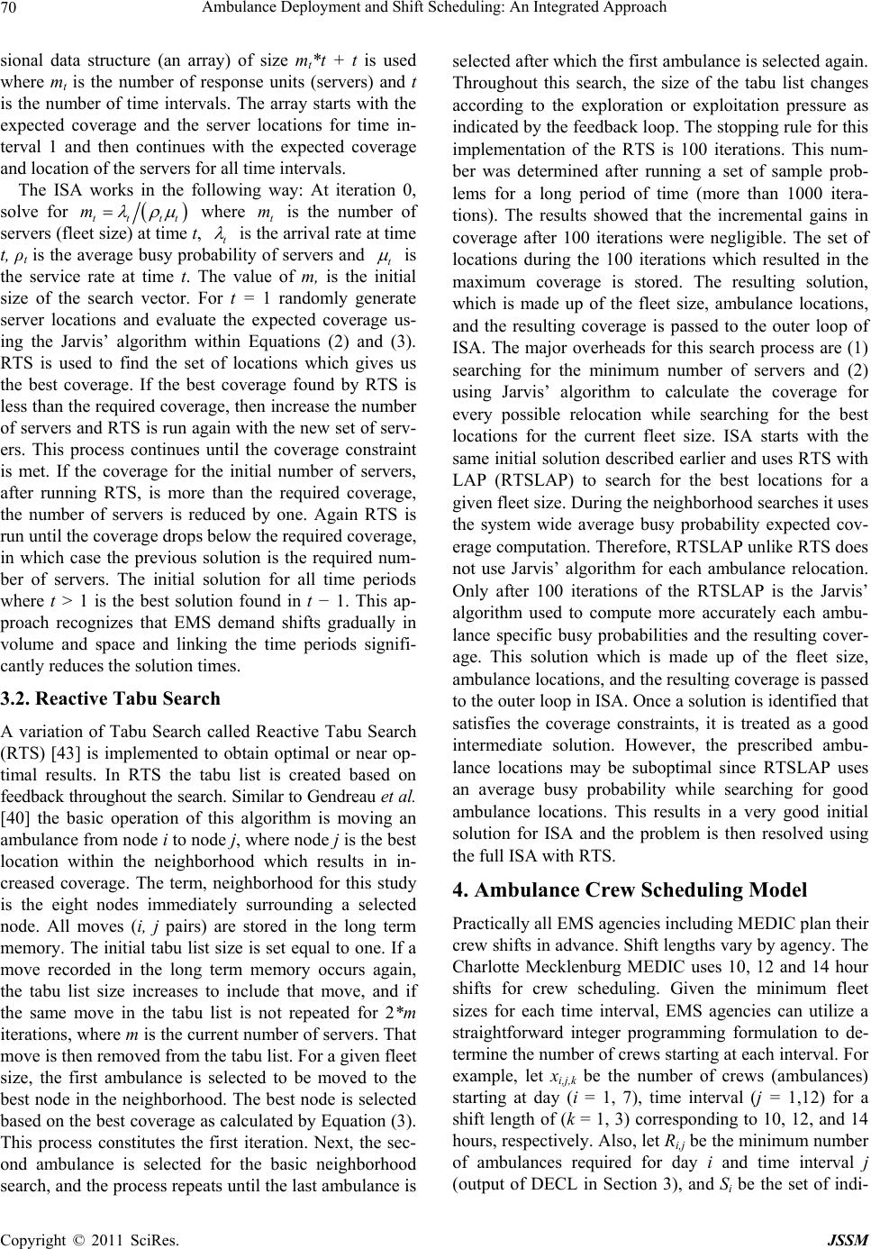 Ambulance Deployment and Shift Scheduling: An Integrated Approach 70 sional data structure (an array) of size mt*t + t is used where mt is the number of response units (servers) and t is the number of time intervals. The array starts with the expected coverage and the server locations for time in- terval 1 and then continues with the expected coverage and location of the servers for all time intervals. The ISA works in the following way: At iteration 0, solve for tttt m where t is the number of servers (fleet size) at time t, t m is the arrival rate at time t, ρt is the average busy probability of servers and t is the service rate at time t. The value of m, is the initial size of the search vector. For t = 1 randomly generate server locations and evaluate the expected coverage us- ing the Jarvis’ algorithm within Equations (2) and (3). RTS is used to find the set of locations which gives us the best coverage. If the best coverage found by RTS is less than the required coverage, then increase the number of servers and RTS is run again with the new set of serv- ers. This process continues until the coverage constraint is met. If the coverage for the initial number of servers, after running RTS, is more than the required coverage, the number of servers is reduced by one. Again RTS is run until the coverage drops below the required coverage, in which case the previous solution is the required num- ber of servers. The initial solution for all time periods where t > 1 is the best solution found in t − 1. This ap- proach recognizes that EMS demand shifts gradually in volume and space and linking the time periods signifi- cantly reduces the solution times. 3.2. Reactive Tabu Search A variation of Tabu Search called Reactive Tabu Search (RTS) [43] is implemented to obtain optimal or near op- timal results. In RTS the tabu list is created based on feedback throughout the search. Similar to Gendreau et al. [40] the basic operation of this algorithm is moving an ambulance from node i to node j, where node j is the best location within the neighborhood which results in in- creased coverage. The term, neighborhood for this study is the eight nodes immediately surrounding a selected node. All moves (i, j pairs) are stored in the long term memory. The initial tabu list size is set equal to one. If a move recorded in the long term memory occurs again, the tabu list size increases to include that move, and if the same move in the tabu list is not repeated for 2*m iterations, where m is the current number of servers. That move is then removed from the tabu list. For a given fleet size, the first ambulance is selected to be moved to the best node in the neighborhood. The best node is selected based on the best coverage as calculated by Equation (3). This process constitutes the first iteration. Next, the sec- ond ambulance is selected for the basic neighborhood search, and the process repeats until the last ambulance is selected after which the first ambulance is selected again. Throughout this search, the size of the tabu list changes according to the exploration or exploitation pressure as indicated by the feedback loop. The stopping rule for this implementation of the RTS is 100 iterations. This num- ber was determined after running a set of sample prob- lems for a long period of time (more than 1000 itera- tions). The results showed that the incremental gains in coverage after 100 iterations were negligible. The set of locations during the 100 iterations which resulted in the maximum coverage is stored. The resulting solution, which is made up of the fleet size, ambulance locations, and the resulting coverage is passed to the outer loop of ISA. The major overheads for this search process are (1) searching for the minimum number of servers and (2) using Jarvis’ algorithm to calculate the coverage for every possible relocation while searching for the best locations for the current fleet size. ISA starts with the same initial solution described earlier and uses RTS with LAP (RTSLAP) to search for the best locations for a given fleet size. During the neighborhood searches it uses the system wide average busy probability expected cov- erage computation. Therefore, RTSLAP unlike RTS does not use Jarvis’ algorithm for each ambulance relocation. Only after 100 iterations of the RTSLAP is the Jarvis’ algorithm used to compute more accurately each ambu- lance specific busy probabilities and the resulting cover- age. This solution which is made up of the fleet size, ambulance locations, and the resulting coverage is passed to the outer loop in ISA. Once a solution is identified that satisfies the coverage constraints, it is treated as a good intermediate solution. However, the prescribed ambu- lance locations may be suboptimal since RTSLAP uses an average busy probability while searching for good ambulance locations. This results in a very good initial solution for ISA and the problem is then resolved using the full ISA with RTS. 4. Ambulance Crew Scheduling Model Practically all EMS agencies including MEDIC plan their crew shifts in advance. Shift lengths vary by agency. The Charlotte Mecklenburg MEDIC uses 10, 12 and 14 hour shifts for crew scheduling. Given the minimum fleet sizes for each time interval, EMS agencies can utilize a straightforward integer programming formulation to de- termine the number of crews starting at each interval. For example, let xi,j,k be the number of crews (ambulances) starting at day (i = 1, 7), time interval (j = 1,12) for a shift length of (k = 1, 3) corresponding to 10, 12, and 14 hours, respectively. Also, let Ri,j be the minimum number of ambulances required for day i and time interval j (output of DECL in Section 3), and Si be the set of indi- Copyright © 2011 SciRes. JSSM  Ambulance Deployment and Shift Scheduling: An Integrated Approach 71 ces in which shifts are active at time interval j, then the scheduling model can be written as: Minimize 7123 ,, 111 ijk ijk x (6) Subject to: 73 ,, , 11 , i ijk ij ijSk Ri j (7) ,, 0, 1,2, ijk x (8) The objective (6) minimizes the number of ambu- lances in each shift starting at one of the 84 time intervals in the week. Equation (7) ensures that in each of the 84 time intervals there are at least the required number of ambulances which are generated by the DECL model. An interesting observation is that when the objective func- tion (6) simply minimizes the sum number of shifts which implies that 10, 12 and 14 hour shifts are weighted equally. Consequently the model is likely to allocate as many ambulances as possible to 14 hour shifts and utilize the 12 and 10 hour shifts as needed. A more versatile ap- proach can be modeled by weighting the three shifts. For example, one can reflect the shift lengths by using 1, 1.2, and 1.4 as weights for the 10, 12 and 14 hour shifts, re- spectively. Let wk be the weight for shift k. Minimize 7123 ,, 111 kijk ijk wx (9) Subject to: 73 ,, , 11 , i ijk ij ijSk Ri j (10) ,, 0, 1,2, ijk x (11) In the formulation above, it is assumed that crews (ambulances) can start their shifts at the beginning of any of the 84 time intervals in the week. In reality, the shift starting times is likely to be far fewer, perhaps only 4 times a day, hence 28 times a week, which reduces the problem size. Regardless, such scheduling formulations can be easily setup in Excel and solved via off-the-shelf solvers, thus increasing the likelihood of user acceptance [44] of our two-stage solution. 5. Computational Experiments Since the first stage requires a heuristic solution ap- proach, the DECL is tested on two important metrics: 1) quality of solutions, and 2) CPU times. The quality of a solution is determined by the minimum number of serv- ers and the coverage. The second metric is simply the CPU time for the ISA. The experiments were performed on a Dell PC Pentium IV 2.4 MHz with 512 MB RAM. The ISA with RTS and ISA with RTSLAP were coded in Java (jdk 1.4). To generate sample problems a hypo- thetical city spanning 1,024 square miles (32 × 32) was created with its regions divided into 64 and 256 demand nodes, representing medium and large scale problem sizes. Two distinct periods of demand patterns are as- sumed. During the first time period the demand is somewhat evenly (uniformly) distributed across the re- gion and during the second time period the demand is non-uniformly distributed, reflecting a shift in call (de- mand) volume due to the migration of population from residential areas of the region to employment, and per- haps, education centers in the region. Ten problem in- stances are randomly generated for each of the 64-zone and 256-zone configurations, comprising the 20 test pro- blems. The results from the 20 problems solved using ISA with RTS and ISA with RTSLAP are summarized in Ta- ble 1. Expected coverage over all runs for each problem size show that the model along with two solution ap- proaches met or exceeded the required coverage of 95% with minimum fleet sizes. LAP adds an extra layer of search to help the ISA start from a “near optimal” point, and therefore the improvements in CPU times are mar- ginal, but it often generates a better final solution, with respect to maintaining coverage with fewer ambulances. The frequency count in Table 1 shows that LAP gener- ates the same number of servers for 22 of the 40 prob- lems instances and better (smaller fleet size) solution quality for 16 of the 40 problem instances. In summary, the DECL is a realistic model but is computationally challenging. Our experimental results show that DECL can be solved effectively and efficiently, therefore it can be successfully embedded in an inte- grated solution package to streamline the complex and tedious series of decisions EMS administrators must make. 6. Analysis of a Case Study The two-stage solution approach was tested with real data from Mecklenburg County (Greater Charlotte), North Carolina. For this experiment twelve, 2-hour time intervals were chosen because Charlotte Mecklenburg MEDIC’s preferred shift durations for ambulance crews are 10, 12, and 14 hours, respectively. Table 2 displays the yearly demand for each of the 2-hour time intervals. We divided the region into 2 mile by 2 mile square nodes (zones). This generated a total of 168 demand nodes, and we as- sumed that the ambulances can be posted in any one of the nodes with the exception of the nodes that make up the outside boundary. In fact, most of the boundary nodes Copyright © 2011 SciRes. JSSM 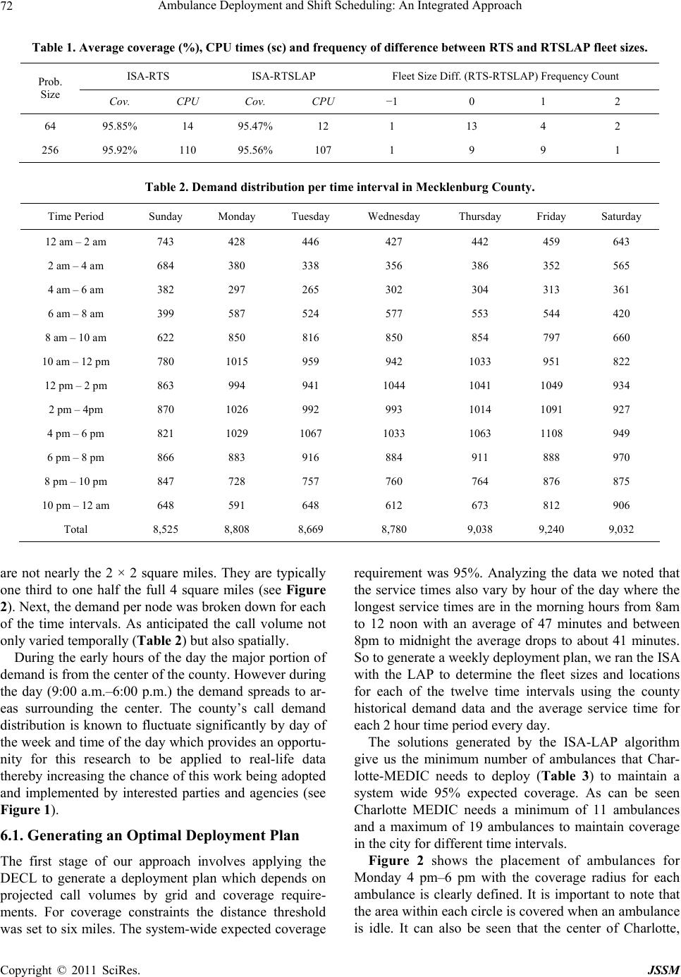 Ambulance Deployment and Shift Scheduling: An Integrated Approach Copyright © 2011 SciRes. JSSM 72 Table 1. Average coverage (%), CPU times (sc) and frequency of difference between RTS and RTSLAP fleet sizes. ISA-RTS ISA-RTSLAP Fleet Size Diff. (RTS-RTSLAP) Frequency Count Prob. Size Cov. CPU Cov. CPU −1 0 1 2 64 95.85% 14 95.47% 12 1 13 4 2 256 95.92% 110 95.56% 107 1 9 9 1 Table 2. Demand distribution per time interval in Mecklenburg County . Time Period Sunday Monday Tuesday Wednesday Thursday Friday Saturday 12 am – 2 am 743 428 446 427 442 459 643 2 am – 4 am 684 380 338 356 386 352 565 4 am – 6 am 382 297 265 302 304 313 361 6 am – 8 am 399 587 524 577 553 544 420 8 am – 10 am 622 850 816 850 854 797 660 10 am – 12 pm 780 1015 959 942 1033 951 822 12 pm – 2 pm 863 994 941 1044 1041 1049 934 2 pm – 4pm 870 1026 992 993 1014 1091 927 4 pm – 6 pm 821 1029 1067 1033 1063 1108 949 6 pm – 8 pm 866 883 916 884 911 888 970 8 pm – 10 pm 847 728 757 760 764 876 875 10 pm – 12 am 648 591 648 612 673 812 906 Total 8,525 8,808 8,669 8,780 9,038 9,240 9,032 are not nearly the 2 × 2 square miles. They are typically one third to one half the full 4 square miles (see Figure 2). Next, the demand per node was broken down for each of the time intervals. As anticipated the call volume not only varied temporally (Table 2) but also spatially. During the early hours of the day the major portion of demand is from the center of the county. However during the day (9:00 a.m.–6:00 p.m.) the demand spreads to ar- eas surrounding the center. The county’s call demand distribution is known to fluctuate significantly by day of the week and time of the day which provides an opportu- nity for this research to be applied to real-life data thereby increasing the chance of this work being adopted and implemented by interested parties and agencies (see Figure 1). 6.1. Generating an Optimal Deployment Plan The first stage of our approach involves applying the DECL to generate a deployment plan which depends on projected call volumes by grid and coverage require- ments. For coverage constraints the distance threshold was set to six miles. The system-wide expected coverage requirement was 95%. Analyzing the data we noted that the service times also vary by hour of the day where the longest service times are in the morning hours from 8am to 12 noon with an average of 47 minutes and between 8pm to midnight the average drops to about 41 minutes. So to generate a weekly deployment plan, we ran the ISA with the LAP to determine the fleet sizes and locations for each of the twelve time intervals using the county historical demand data and the average service time for each 2 hour time period every day. The solutions generated by the ISA-LAP algorithm give us the minimum number of ambulances that Char- lotte-MEDIC needs to deploy (Table 3) to maintain a system wide 95% expected coverage. As can be seen Charlotte MEDIC needs a minimum of 11 ambulances and a maximum of 19 ambulances to maintain coverage in the city for different time intervals. Figure 2 shows the placement of ambulances for Monday 4 pm–6 pm with the coverage radius for each ambulance is clearly defined. It is important to note that the area within each circle is covered when an ambulance is idle. It can also be seen that the center of Charlotte, 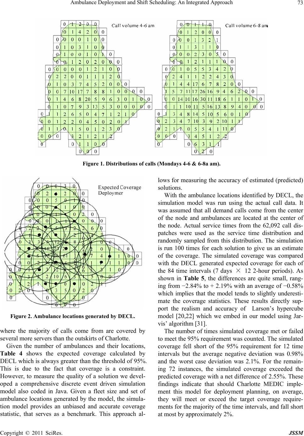 Ambulance Deployment and Shift Scheduling: An Integrated Approach 73 Figure 1. Distributions of calls (Mondays 4-6 & 6-8a am). Figure 2. Ambulance locations generated by DECL. where the majority of calls come from are covered by several more servers than the outskirts of Charlotte. Given the number of ambulances and their locations, Table 4 shows the expected coverage calculated by DECL which is always greater than the threshold of 95%. This is due to the fact that coverage is a constraint. However, to measure the quality of a solution we devel- oped a comprehensive discrete event driven simulation model also coded in Java. Given a fleet size and set of ambulance locations generated by the model, the simula- tion model provides an unbiased and accurate coverage statistic, that serves as a benchmark. This approach al- lows for measuring the accuracy of estimated (predicted) solutions. With the ambulance locations identified by DECL, the simulation model was run using the actual call data. It was assumed that all demand calls come from the center of the node and ambulances are located at the center of the node. Actual service times from the 62,092 call dis- patches were used as the service time distribution and randomly sampled from this distribution. The simulation is run 100 times for each solution to give us an estimate of the coverage. The simulated coverage was compared with the DECL generated expected coverage for each of the 84 time intervals (7 days × 12 2-hour periods). As shown in Table 5, the differences are quite small, rang- ing from −2.84% to + 2.19% with an average of −0.58% which implies that the model tends to slightly underesti- mate the coverage statistics. These results directly sup- port the realism and accuracy of Larson’s hypercube model [20,22] which we embed in our model using Jar- vis’ algorithm [31]. The number of times simulated coverage met or failed to meet the 95% requirement was counted. The simulated coverage fell short of the 95% requirement for 12 time intervals but the average negative deviation was 0.98% and the worst case deviation was 2.1%. For the remain- ing 72 instances, the simulated coverage exceeded the predicted coverage with a net difference of 2.55%. These findings indicate that should Charlotte MEDIC imple- ment this model for deployment planning, on average, they will meet or exceed the target coverage require- ments for the majority of the time intervals, and fall short t most by approximately 2%. a Copyright © 2011 SciRes. JSSM 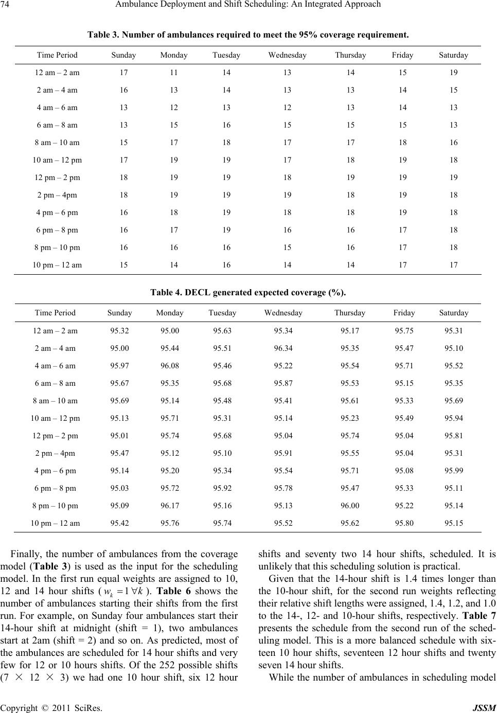 Ambulance Deployment and Shift Scheduling: An Integrated Approach 74 Table 3. Number of ambulances required to meet the 95% coverage requirement. Time Period Sunday Monday Tuesday Wednesday Thursday Friday Saturday 12 am – 2 am 17 11 14 13 14 15 19 2 am – 4 am 16 13 14 13 13 14 15 4 am – 6 am 13 12 13 12 13 14 13 6 am – 8 am 13 15 16 15 15 15 13 8 am – 10 am 15 17 18 17 17 18 16 10 am – 12 pm 17 19 19 17 18 19 18 12 pm – 2 pm 18 19 19 18 19 19 19 2 pm – 4pm 18 19 19 19 18 19 18 4 pm – 6 pm 16 18 19 18 18 19 18 6 pm – 8 pm 16 17 19 16 16 17 18 8 pm – 10 pm 16 16 16 15 16 17 18 10 pm – 12 am 15 14 16 14 14 17 17 Table 4. DECL generated expected coverage (%). Time Period Sunday Monday Tuesday Wednesday Thursday Friday Saturday 12 am – 2 am 95.32 95.00 95.63 95.34 95.17 95.75 95.31 2 am – 4 am 95.00 95.44 95.51 96.34 95.35 95.47 95.10 4 am – 6 am 95.97 96.08 95.46 95.22 95.54 95.71 95.52 6 am – 8 am 95.67 95.35 95.68 95.87 95.53 95.15 95.35 8 am – 10 am 95.69 95.14 95.48 95.41 95.61 95.33 95.69 10 am – 12 pm 95.13 95.71 95.31 95.14 95.23 95.49 95.94 12 pm – 2 pm 95.01 95.74 95.68 95.04 95.74 95.04 95.81 2 pm – 4pm 95.47 95.12 95.10 95.91 95.55 95.04 95.31 4 pm – 6 pm 95.14 95.20 95.34 95.54 95.71 95.08 95.99 6 pm – 8 pm 95.03 95.72 95.92 95.78 95.47 95.33 95.11 8 pm – 10 pm 95.09 96.17 95.16 95.13 96.00 95.22 95.14 10 pm – 12 am 95.42 95.76 95.74 95.52 95.62 95.80 95.15 Finally, the number of ambulances from the coverage model (Table 3) is used as the input for the scheduling model. In the first run equal weights are assigned to 10, 12 and 14 hour shifts (). Table 6 shows the number of ambulances starting their shifts from the first run. For example, on Sunday four ambulances start their 14-hour shift at midnight (shift = 1), two ambulances start at 2am (shift = 2) and so on. As predicted, most of the ambulances are scheduled for 14 hour shifts and very few for 12 or 10 hours shifts. Of the 252 possible shifts (7 × 12 × 3) we had one 10 hour shift, six 12 hour shifts and seventy two 14 hour shifts, scheduled. It is unlikely that this scheduling solution is practical. 1 k w Given that the 14-hour shift is 1.4 times longer than the 10-hour shift, for the second run weights reflecting their relative shift lengths were assigned, 1.4, 1.2, and 1.0 to the 14-, 12- and 10-hour shifts, respectively. Table 7 presents the schedule from the second run of the sched- uling model. This is a more balanced schedule with six- teen 10 hour shifts, seventeen 12 hour shifts and twenty seven 14 hour shifts. k While the number of ambulances in scheduling model Copyright © 2011 SciRes. JSSM 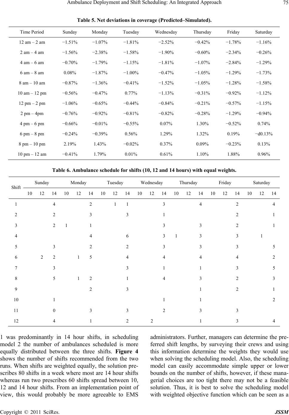 Ambulance Deployment and Shift Scheduling: An Integrated Approach 75 Table 5. Net deviations in coverage (Predicted–Simulated). Time Period Sunday Monday Tuesday Wednesday Thursday Friday Saturday 12 am – 2 am −1.51% −1.07% −1.81% −2.52% −0.42% −1.78% −1.16% 2 am – 4 am −1.56% −2.38% −1.58% −1.90% −0.60% −2.34% −0.26% 4 am – 6 am −0.70% −1.79% −1.15% −1.81% −1.07% −2.84% −1.29% 6 am – 8 am 0.08% −1.87% −1.00% −0.47% −1.05% −1.29% −1.73% 8 am – 10 am −0.87% −1.36% −0.41% −1.52% −1.05% −1.28% −1.58% 10 am – 12 pm −0.56% −0.47% 0.77% −1.13% −0.31% −0.92% −1.12% 12 pm – 2 pm −1.06% −0.65% −0.44% −0.84% −0.21% −0.57% −1.15% 2 pm – 4pm −0.76% −0.92% −0.81% −0.82% −0.28% −1.29% −0.94% 4 pm – 6 pm −0.66% −0.01% −0.55% 0.07% 1.30% −0.52% 0.74% 6 pm – 8 pm −0.24% −0.39% 0.56% 1.29% 1.32% 0.19% −d0.13% 8 pm – 10 pm 2.19% 1.43% −0.02% 0.37% 0.09% −0.23% 0.13% 10 pm – 12 am −0.41% 1.79% 0.01% 0.61% 1.10% 1.88% 0.96% Table 6. Ambulance schedule for shifts (10, 12 and 14 hours) w i th equal weights. Sunday Monday Tuesday Wednesday Thursday Friday Saturday Shift 10 12 14 10 12 14 10 12 14 1012 1410 12 14 10 12 14 10 12 14 1 4 2 1 1 3 4 2 4 2 2 3 3 1 2 1 3 2 1 1 3 3 2 1 4 4 6 3 1 3 3 1 5 3 2 2 3 3 3 5 6 2 2 1 5 4 4 4 4 2 7 3 3 1 1 3 5 8 5 1 2 1 4 3 2 3 9 2 3 1 2 1 10 1 1 1 2 11 0 3 3 2 3 3 12 4 1 2 2 1 3 4 1 was predominantly in 14 hour shifts, in scheduling model 2 the number of ambulances scheduled is more equally distributed between the three shifts. Figure 4 shows the number of shifts recommended from the two runs. When shifts are weighted equally, the solution pre- scribes 80 shifts in a week where most are 14 hour shifts whereas run two prescribes 60 shifts spread between 10, 12 and 14 hour shifts. From an implementation point of view, this would probably be more agreeable to EMS administrators. Further, managers can determine the pre- ferred shift lengths, by surveying their crews and using this information determine the weights they would use when solving the scheduling model. Also, the scheduling model can easily accommodate simple upper or lower bounds on the number of shifts, however, if these mana- gerial choices are too tight there may not be a feasible solution. Thus, it is best to solve the scheduling model with weighted objective function which can be seen as a Copyright © 2011 SciRes. JSSM 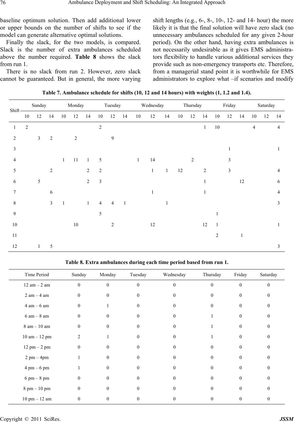 Ambulance Deployment and Shift Scheduling: An Integrated Approach 76 baseline optimum solution. Then add additional lower or upper bounds on the number of shifts to see if the model can generate alternative optimal solutions. Finally the slack, for the two models, is compared. Slack is the number of extra ambulances scheduled above the number required. Table 8 shows the slack from run 1. There is no slack from run 2. However, zero slack cannot be guaranteed. But in general, the more varying shift lengths (e.g., 6-, 8-, 10-, 12- and 14- hour) the more likely it is that the final solution will have zero slack (no unnecessary ambulances scheduled for any given 2-hour period). On the other hand, having extra ambulances is not necessarily undesirable as it gives EMS administra- tors flexibility to handle various additional services they provide such as non-emergency transports etc. Therefore, from a managerial stand point it is worthwhile for EMS administrators to explore what –if scenarios and modify Table 7. Ambulance schedule for shifts (10, 12 and 14 hours) with weights (1, 1.2 and 1.4). Sunday Monday Tuesday Wednesday Thursday Friday Saturday Shift 10 12 14 10 12 14 10 12 1410121410 12 14 10 12 14 10 12 14 1 2 2 1 10 4 4 2 3 2 2 9 3 1 1 4 1 11 1 5 1 14 2 3 5 2 2 2 1 1 12 2 3 4 6 5 2 3 1 12 6 7 6 1 1 4 8 3 1 1 4 4 1 1 3 9 5 1 10 10 2 12 121 1 11 2 1 12 1 5 3 Table 8. Extra ambulances during eac h time per iod based from run 1. Time Period Sunday Monday Tuesday Wednesday Thursday Friday Saturday 12 am – 2 am 0 0 0 0 0 0 0 2 am – 4 am 0 0 0 0 0 0 0 4 am – 6 am 0 1 0 0 0 0 0 6 am – 8 am 0 0 0 0 1 0 0 8 am – 10 am 0 0 0 0 1 0 0 10 am – 12 pm 2 1 0 0 1 0 0 12 pm – 2 pm 0 0 0 0 0 0 0 2 pm – 4pm 1 0 0 0 0 0 0 4 pm – 6 pm 1 0 0 0 0 0 0 6 pm – 8 pm 0 0 0 0 0 0 0 8 pm – 10 pm 0 0 0 0 0 0 0 10 pm – 12 am 0 0 0 0 0 0 0 Copyright © 2011 SciRes. JSSM  Ambulance Deployment and Shift Scheduling: An Integrated Approach 77 ing the weights in the scheduling model to generate al- ternative schedules to handle different situations. 7. Conclusions In this paper we developed a two-stage comprehensive solution approach to solving the ambulance deployment and personnel scheduling problem for EMS administra- tors. The first stage utilizes a realistic model for dynamic environments with the objective of deploying the mini- mum number of ambulances required to meet mandated coverage requirements. A search algorithm was devel- oped and tested for efficiency and effectiveness. Compu- tational findings showed that the model and the algo- rithm are consistent, fast and provide optimal or near optimal solutions. To further test the realism of our model we utilized EMS call data from Charlotte, North Carolina and validated our findings using a discrete event simula- tion. Comparisons with the simulation model show that our predicted coverage statistics are on average quite accurate with less than 1% net average deviation. For the second stage two variations of the scheduling model was formulated and applied to the case study. The shift scheduling model is shown to be both practical and flexible giving managers the opportunity to reflect shift length preference of their personnel. This integrated approach is a viable alternative to making deployment decisions and developing crew sche- dules independently, manually or aided by software. To the best of our knowledge, while the existing EMS crew scheduling software are very user friendly allowing crews to sign up for their preferred shifts, they do not optimize any objective. What is lacking from the com- mercially available software are the integrated (two-stage) deployment and crew scheduling models. Solution from the scheduling model should be the starting screen for the commercially available EMS crew scheduling software. As shown above, solutions with multiple shift lengths weighted according to their shift lengths will generate minimum slack solutions. There are a number of directions for future studies. For example, in our model the expected coverage require- ment is a hard constraint. Future studies might treat the coverage requirement as a goal constraint while penaliz- ing negative deviations from the coverage requirement with an exponential function. Given a deployment plan, it would be interesting to compare the crew schedules generated manually or via commercial software to those from the scheduling models generated from this work. REFERENCES [1] NFPA 1720, “Standard for the Organization and De- ployment of Fire Suppression Operations, Emergency Medical Operations and Special Operations to the Public by Volunteer Fire Departments,” 2010 Ed., NFPA, Quincy, 2010. [2] D. M. Williams and M. Ragone, “2009 JEMS 200-City Survey: Zeroing in on What Matters,” Journal of Emer- gency Medical Services, Vol. 34, No. 2, 2010, pp. 38-42. [3] H. Setzler, C. Saydam and S. Park, “EMS Call Volume Predictions: A Comparative Study,” Computers & Op- erations Research, Vol. 36, No. 6, 2009, pp. 1843-1851. doi:10.1016/j.cor.2008.05.010 [4] ILOG, “ILOG Cplex 7.0 Reference Manual,” ILOG, 2000. [5] R. D. Galvao, F. Y. Chiyoshi and R. Morabito, “Towards Unified Formulations and Extensions of Two Classical Probabilistic Location Models,” Computers & Operations Research, Vol. 32, No. 1, 2005, pp. 15-33. doi:10.1016/S0305-0548(03)00200-4 [6] O. Karasakal and E. K. Karasakal, “A Maximal Covering Location Model in the Presence of Partial Coverage,” Computers & Operations Research, Vol. 31, No. 9, 2004, pp. 1515-1526. doi:10.1016/S0305-0548(03)00105-9 [7] J. B. Goldberg, “Operations Research Models for the Deployment of Emergency Services Vehicles,” EMS Management Journal, Vol. 1, No. 1, 2004, pp. 20-39. [8] L. Brotcorne, G. Laporte and F. Semet, “Fast Heuristics for Large Scale Covering Location Problems,” Computers & Operations Research, Vol. 29, No. 6, 2002, pp. 651-665. doi:10.1016/S0305-0548(99)00088-X [9] H. Aytug and C. Saydam, “Solving Large-Scale Maxi- mum Expected Covering Location Problems by Genetic Algorithms: A Comparative Study,” European Journal of Operational Research, Vol. 141, No. 3, 2002, pp. 480-494. doi:10.1016/S0377-2217(01)00260-0 [10] C. Saydam and H. Aytug, “Accurate Estimation of Ex- pected Coverage: Revisited,” Socio-Economic Planning Sciences, Vol. 37, No. 1, 2003, pp. 69-80. doi:10.1016/S0038-0121(02)00004-6 [11] M. Gendreau, G. Laporte and F. Semet, “A Dynamic Model and Parallel Tabu Search Heuristic for Real Time Ambulance Relocation,” Parallel Computing, Vol. 27, No. 12, 2001, pp. 1641-1653. doi:10.1016/S0167-8191(01)00103-X [12] D. A. Schilling, V. Jayaraman and R. Barkhi, “A Review of Covering Problems in Facility Location,” Location Sci- ence, Vol. 1, No. 1, 1993, pp. 25-55. [13] S. H. Owen and M. S. Daskin, “Strategic Facility Loca- tion: A Review,” European Journal of Operational Re- search, Vol. 111, No. 3, 1998, pp. 423-447. doi:10.1016/S0377-2217(98)00186-6 [14] L. Brotcorne, G. Laporte and F. Semet, “Ambulance Lo- cation and Relocation Models,” European Journal of Op- erational Research, Vol. 147, No. 3, 2003, pp. 451-463. doi:10.1016/S0377-2217(02)00364-8 [15] M. S. Daskin, “A Maximal Expected Covering Location Model: Formulation, Properties and Heuristic Solution,” Transportation Science, Vol. 17, No. 1, 1983, pp. 48-69. Copyright © 2011 SciRes. JSSM  Ambulance Deployment and Shift Scheduling: An Integrated Approach 78 doi:10.1287/trsc.17.1.48 [16] C. ReVelle and K. Hogan, “The Maximum Availability Location Problem,” Transportation Science, Vol. 23, No. 3, 1989, pp. 192-200. doi:10.1287/trsc.23.3.192 [17] M. O. Ball and L. F. Lin, “A Reliability Model Applied to Emergency Service Vehicle Location,” Operations Re- search, Vol. 41, No. 1, 1993, pp. 18-36. doi:10.1287/opre.41.1.18 [18] C. ReVelle and K. Hogan, “The Maximum Reliability Location Problem and Alpha-Reliable P-Center Problems: Derivatives of the Probabilistic Location Set Covering Problem,” Annals of Operations Research, Vol. 18, No. 1, 1989, pp. 155-174. doi:10.1007/BF02097801 [19] V. Marianov and C. ReVelle, “The Queuing Probabilistic Location Set Covering Problem and Some Extensions,” Socio-Economic Planning Sciences, Vol. 28, No. 3, 1994, pp. 167-178. doi:10.1016/0038-0121(94)90003-5 [20] R. C. Larson, “A Hypercube Queuing Model for Facility Location and Redistricting in Urban Emergency Ser- vices,” Computers & Operations Research, Vol. 1, No. 1, 1974, pp. 67-95. doi:10.1016/0305-0548(74)90076-8 [21] A. S. Zaki, H. K. Cheng and B. R. Parker, “A Simulation Model for the Analysis and Management of An Emer- gency Service System,” Socio-Economic Planning Sci- ences, Vol. 31, No. 3, 1997, pp. 173-189. doi:10.1016/S0038-0121(97)00013-X [22] R. C. Larson, “Approximating the Performance of Urban Emergency Service Systems,” Operations Research, Vol. 23, No. 5, 1975, pp. 845-868. doi:10.1287/opre.23.5.845 [23] R. Batta, J. M. Dolan, and N. N. Krishnamurthy, “The Maximal Expected Covering Location Problem: Revis- ited,” Transportation Science, Vol. 23, No. 4, 1989, pp. 277-287. doi:10.1287/trsc.23.4.277 [24] Y. Chan, “Location Theory and Decision Analysis,” South Western College Publishing, Cincinnati, 2001. [25] M. S. Daskin, “Network and Discrete Location,” John Wiley & Sons Inc., New York, 1995. [26] R. C. Larson and A. R. Odoni “Urban Operations Re- search,” Prentice-Hall, Englewood Cliffs, 1981. [27] C. ReVelle, “Review, Extension and Prediction in Emer- gency Siting Models,” European Journal of Operational Research, Vol. 40, No. 1, 1989, pp. 58-69. doi:10.1016/0377-2217(89)90272-5 [28] C. Saydam, J. Repede and T. Burwell, “Accurate Estima- tion of Expected Coverage: A Comparative Study,” Socio-Economic Planning Sciences, Vol. 28, No. 2, 1994, pp. 113-120. doi:10.1016/0038-0121(94)90010-8 [29] T. H. Burwell, J. P. Jarvis and M. A. McKnew, “Model- ing Co-Located Servers and Dispatch Ties in the Hyper- cube Model,” Computers & Operations Research, Vol. 20, No. 1993, pp. 113-119. [30] R. A. Takeda, J. A. Widmer and R. Morabito, “Analysis of Ambulance Decentralization in an Urban Medical Emergency Service Using the Hypercube Queuing Model.,” Computers & Operations Research, Vol. 34, No. 3, 2007, pp. 727-741. doi:10.1016/j.cor.2005.03.022 [31] J. P. Jarvis, “Approximating the Equilibrium Behavior of Multi-Server Loss Systems,” Management Science, Vol. 31, No. 2, 1985, pp. 235-239. doi:10.1287/mnsc.31.2.235 [32] J. Penner, “Interview with the Charlotte MEDIC Direc- tor,” H. K. Rajagopalan, 2004. [33] J. Repede and J. Bernardo, “Developing and Validating a Decision Support System for Locating Emergency Mdei- cal Vehichles in Lousville, Kentucky,” European Journal of Operational Research, Vol. 75, No. 3, 1994, pp. 567-581. doi:10.1016/0377-2217(94)90297-6 [34] P. Trudeau, J. M. Rousseau, J. A. Ferland and J. Cho- quette, “An Operations Research Approach for the Plan- ning and Operation of an Ambulance Service,” INFOR, Vol. 27, No. 1, 1989, pp. 95-113. [35] G. Erdogan, E. Erkut, A. Ingolfsson and G. Laporte, “Scheduling Ambulance Crews for Maximum Coverage,” Journal of Operational Research Society, Vol. 61, No. 4, 2010, pp. 543-550. doi:10.1057/jors.2008.163 [36] Y. Li and E. Kozan, “Rostering Ambulance Services,” Industrial Engineering and Management Society, Kita- kyushu, Japan, 2009, pp. 14-16. [37] V. Marianov and C. ReVelle, “The Queueing Maximal Availability Location Problem: A Model for Siting of Emergency Vehicles,” European Journal of Operational Research, Vol. 93, No. 1, 1996, pp. 110-120. doi:10.1016/0377-2217(95)00182-4 [38] J. E. Beasley and P. C. Chu, “A Genetic Algorithm for the Set Covering Problem,” European Journal of Opera- tional Research, Vol. 94, No. 2, 1996, pp. 392-404. doi:10.1016/0377-2217(95)00159-X [39] S. Benati and G. Laporte, “Tabu Search Algorithms for the (r|Xp)-Medianoid and (r|p) Centroid Problems,” Lo- cation Science, Vol. 2, No. 4, 1994, pp. 193-204. [40] M. Gendreau, G. Laporte and F. Semet, “Solving an Ambulance Location Model by Tabu Search,” Location Science, Vol. 5, No. 2, 1997, pp. 75-88. doi:10.1016/S0966-8349(97)00015-6 [41] J. Jaramillo, J. Bhadury and R. Batta, “On the Use of Genetic Algorithms to Solve Location Problems,” Com- puters & Operations Research, Vol. 29, No. 6, 2002, pp. 761-779. doi:10.1016/S0305-0548(01)00021-1 [42] H. K. Rajagopalan, F. E. Vergara, C. Saydam and J. Xiao, “Developing Effective Meta-Heuristics For A Probabilis- tic Location Model Via Experimental Design,” European Journal of Operational Research, Vol. 177, No. 2, 2007, pp. 365-377. [43] R. Battiti and G. Tecchiolli, “The Reactive Tabu Search,” Journal on Computing, Vol. 6, No. 2, 1994, pp. 126-140. [44] F. S. Hillier and G. J. Lieberman, “Introduction to Opera- tions Research,” 8th Ed., McGraw Hill, New York, 2005. Copyright © 2011 SciRes. JSSM
|