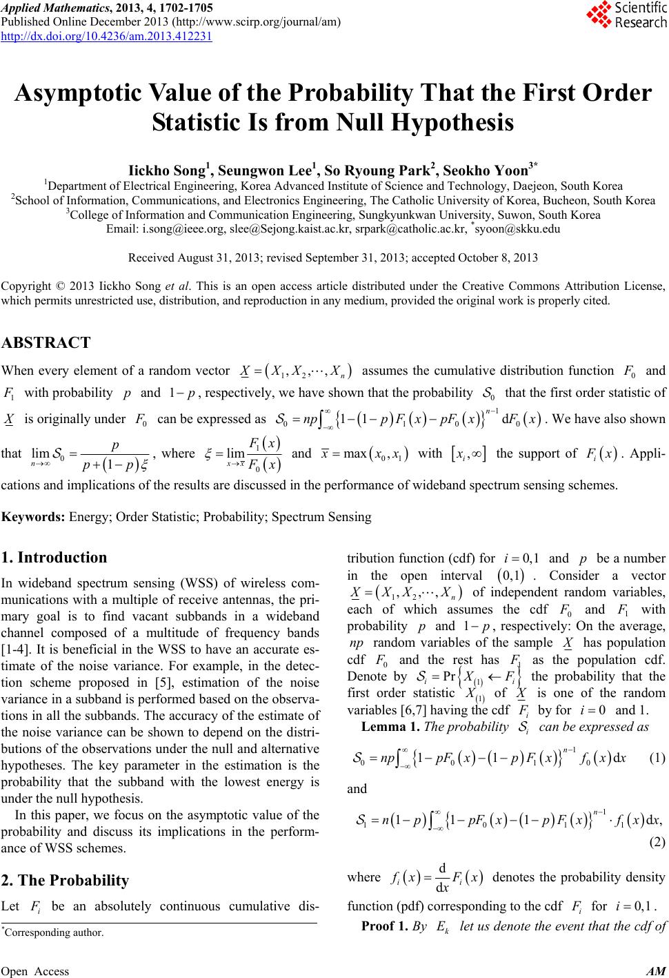
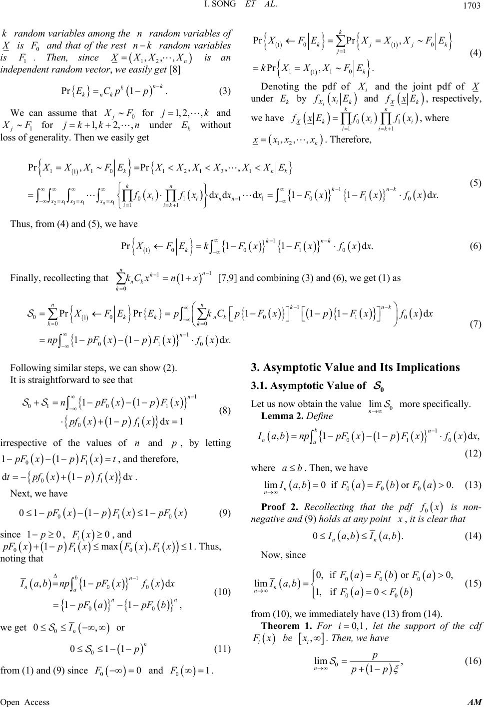
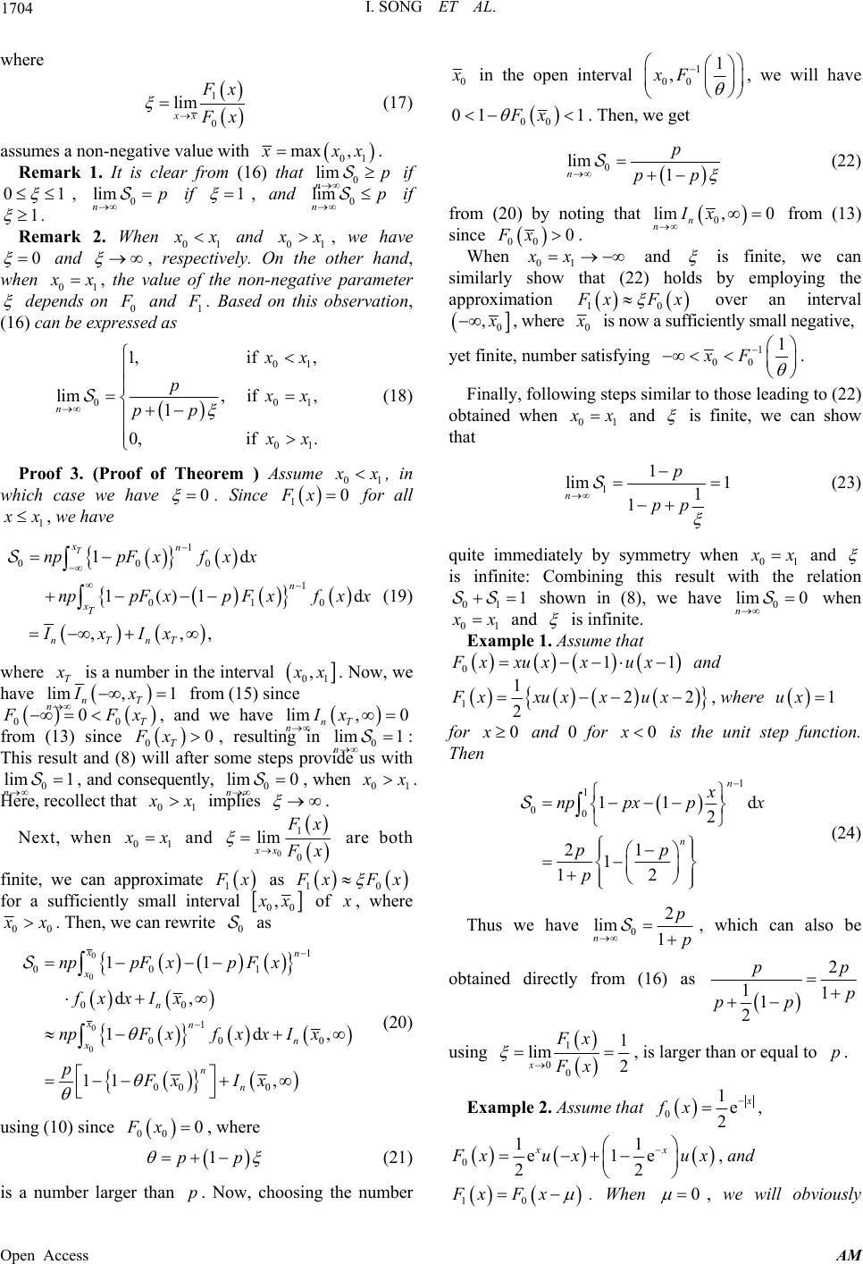
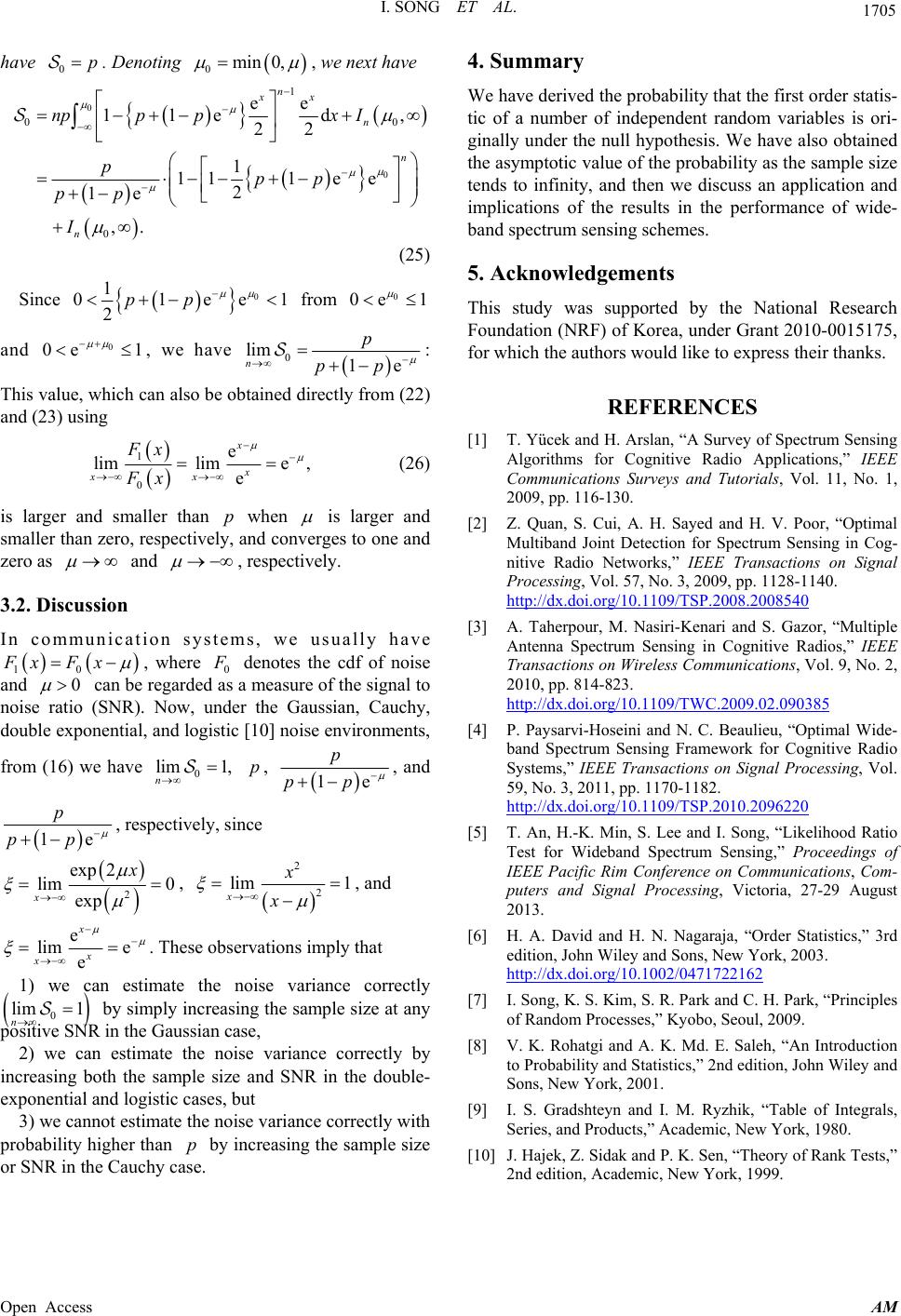
Applied Mathematics, 2013, 4, 1702-1705
Published Online December 2013 (http://www.scirp.org/journal/am)
http://dx.doi.org/10.4236/am.2013.412231
Open Access AM
Asymptotic Value of the Probability That the First Order
Statistic Is from Null Hypothesis
Iickho Song1, Seungwon Lee1, So Ryoung Park2, Seokho Yoon3*
1Department of Electrical Engineering, Korea Advanced Institute of Science and Technology, Daejeon, South Korea
2School of Information, Communications, and Electronics Engineering, The Catholic University of Korea, Bucheon, South Korea
3College of Information and Communication Engineering, Sungkyunkwan University, Suwon, South Korea
Received August 31, 2013; revised September 31, 2013; accepted October 8, 2013
Copyright © 2013 Iickho Song et al. This is an open access article distributed under the Creative Commons Attribution License,
which permits unrestricted use, distribution, and reproduction in any medium, provided the original work is properly cited.
ABSTRACT
When every element of a random vector


12
,,,
n
X
XX X assumes the cumulative distribution function 0
F
and
1
F
with probability and pp

1, respectively, we have shown that the probability that the first order statistic of
0

X
is originally under 0
F
can be expressed as . We have also shown
that
  
010
11 dnppFx pFxFx


 



1n

0

0
lim 1
n
p
pp

 
, where



1
0
lim
xx
F
x
F
x


 and


01
max ,
x
xx with


,
i
x

the support of

i

F
x. Appli-
cations and implications of the results are discussed in the performance of wideband spectrum sensing schemes.
Keywords: Energy; Order Statistic; Probability; Spectrum Sensing
1. Introduction
In wideband spectrum sensing (WSS) of wireless com-
munications with a multiple of receive antennas, the pri-
mary goal is to find vacant subbands in a wideband
channel composed of a multitude of frequency bands
[1-4]. It is beneficial in the WSS to have an accurate es-
timate of the noise variance. For example, in the detec-
tion scheme proposed in [5], estimation of the noise
variance in a subband is performed based on the observa-
tions in all the subbands. The accuracy of the estimate of
the noise variance can be shown to depend on the distri-
butions of the observatio ns under the null and alternative
hypotheses. The key parameter in the estimation is the
probability that the subband with the lowest energy is
under the null hypothesis.
In this paper, we focus on the asymptotic value of the
probability and discuss its implications in the perform-
ance of WSS schemes.
2. The Probability
Let i
F
be an absolutely continuous cumulative dis-
tribution function (cdf) fo r and be a number
in the open interval 0,1ip


0,1 . Consider a vector


12
,,,
n
X
XX X of independent random variables,
each of which assumes the cdf 0
F
and 1 with
probability and 1F
pp

, respectively: On the average,
random variables of the sample
np
X
has population
cdf 0
F
and the rest has as the population cdf.
Denote by 1
F



1
i
Pr i
X
F the probability that the
first order statistic

1
X
of
X
is one of the random
variables [6,7] having the cdf i
F
by for and 1. 0

x
1n
i
1
1
f
 
Fx
Lemma 1. The probability can be expressed as
i

 
11p F
 
Fx

x
10
p

x




n

p
00
pF
11


0
x
1
f
d
1
d,
np

np




(1)
and
 
1xx 
(2)
where

i
d
d
i
f
xFx
x denotes the probability density
function (pdf) corresponding to the cdf i
F
for 0,1i

.
Proof 1. By let us denote the event that the cdf of
k
E
*Corresponding author.

I. SONG ET AL. 1703
k random variables among the random variables of n
X
is 0
F
and that of the rest random variables
is 1
nk
F
. Then, since

12
,,,
n
X
XX
1pp
X is an
independent random vector, we easily get [8]
 
Pr .
nk
k
knk
EC  

0
(3)
We can assume that j
X
F

for and
1j
1, 2,,jk
X
F for under without
loss of generality. Then we easily get
1,jk 2,k,nk E








00
11
1
110
1
PrPr ,
Pr ,.
k
kjj
j
k
k
X
FEXX XFE
kXXXFE

 

 (4)
Denoting the pdf of i
X
and the joint pdf of
X
under by
k
E


k
i
Xi and

Xk

f
xE , respectively,
f
xE
we have

 
01
11
kn
Xk i
iik
i
f
xEfxf x

, where


12
,,,
n
x
xx x. Therefore,




 




2131 1
11 12131 1
1
0111 010
11
,,, ,
dd d11d.
n
knk
kn knk
iinn
xxxxxx iik
XXXFEXXXX XXE

0
rPr P
f
xfxxxxFx Fxfxx
 

 

 





 





(5)
Thus, from (4) and (5) , we ha ve

    
1
0010
Pr11d .
knk
k
FEkF xFxfxx




1
X
(6)
Finally, recollecting that

1
1
0
1
nn
k
n x
k
x
nk
kC




 [7,9] and combining (3 ) and (6), we get (1) as


      
 
kk
 

1
000 10
1
00
1
010
Pr11 1d
11 d.
nn
knk
nk
kk
n
Pr
X
FEpkCpF xpFxfxx
nppF xxfxx
 





 
 

 

 




1
E
F


 
x
p



0
01
11x
f

(7)
Following similar steps, we can show (2).
It is straightforward to see that
 
 
1
01 1
1d
n
npF pFx
pf xpx



 
 


n
x


x
dtp
(8)
irrespective of the values of and , by letting
, and therefore,
.
p

01
11p Fxt
  
01
1fxpf 
pF


dx
Next, we have
 


1x

001
1pFxp FpFx 01
p

(9)
since , , and 10


0
i
Fx
 


01
,Fx
01
1mFxaxx1pFx p F. Thus,
noting that
   
   
,1
11
b
a
nn

00
n1
00
d
,
n
I
a bnppFxxx
pF ab


 
f
p

F (10)
we get

0
0,
n
I or


0
011
n
p
0
(11)
from (1) and (9) since and .

0
F

01F
3. Asymptotic Value and Its Implications
3.1. Asymptotic Value of
0

Let us now obtain the value more specifically.
0
lim
n

Lemma 2. Define
   
1
010
,1 1
bn
nad,
I
abnppFxpFxfxx

 

(12)
where ab

. Then, we have



 
00 0
lim,0 ifor0.
n
nIabFa FbFa 

 (13)
Proof 2. Recollecting that the pdf

0
f
x is non-
negative and (9) holds at any point
x
, it is clear that


0, ,.
I
nn
abI ab (14)
Now, since


 
 
00 0
00
0, ifor0,
lim ,1, if0
n
n
Fa FbFa
Iab Fa Fb





 (15)
from (10), we immediately have (13) from (14).
Theorem 1. For 0,1i

, let the support of the cdf


i
F
x be


,
i
x

. Then, we have

0
lim ,
1
n
p
pp

 
 (16)
Open Access AM

I. SONG ET AL.
1704
where



1
0
lim
xx
F
x
F
x


 (17)
assumes a non-negative value with

01
max ,
x
xx.
Remark 1. It is clear from (16) that if
0
lim
np  
01

, if
0
lim
np  1


, and 0 lim
np 

 if
1

.
Remark 2. When 01
x
x and 01
x
x, we have
0

 and

, respectively. On the other hand,
when 01
x
x, the value of the non-negative parameter

depends on 0
F
and 1
F
. Based on this observation,
(16) can be expresse d as

01
0
01
1,if ,
lim, if,
1
0,if .
n0
1
x
x
p
x
x
pp
x
x










 (18)
Proof 3. (Proof of Theorem ) Assume 10
x
x

, in
which case we have 0

. Since for all

1
Fx 0
1
x
x, we have
  
   

1
000
1
010
1d
1()1
,,,
T
xn
n
xT
nTnT
nppF xfxx
nppFxp Fxfxx
IxIx









d (19)
where T
x
is a number in the interval


01
,
x
x. Now, we
have

lim
n

0
, 1
nT
Ix

from (15) since
0

0T
F
Fx , and we have n

, 0
nT
lim Ix


m1 from (13) since , resulting in 0
n

0
T 0
Fx li


01
:
This result and (8) will after some steps provide us with
0
n , and consequently, 0 n , when lim 1lim 0
x
x.
Here, recollect that 01
x
x implies

.
Next, when 01
x
x and


0
1
0
lim
xx
F
x
F
x


 are both
finite, we can approximate

1
F
x as



10
F
xFx  
for a sufficiently small interval


00
,
x
x of
x
, where
00
x
x. Then, we can rewrite as
0

 





 
  
0
0
0
0
1
001
00
1
000
00 0
11
d,
1d
11 ,
xn
x
n
xn
n
x
n
n
nppFxp Fx
fxxIx
npFxfxxIx
pFx Ix







 







,
(20)
using (10) since , where

00 0Fx

1pp

  (21)
is a number larger than . Now, choosing the number
p
0
x
in the open interval 1
00 1
,xF




 



, we will have


00
01 1Fx 

. Then, we get

0
lim 1
n
p
pp

 
 (22)
from (20) by noting that

0
lim, 0
n
nIx   from (13)
since


00 0Fx.
When 01 xx

 and

is finite, we can
similarly show that (22) holds by employing the
approximation


10
F
xF  x over an interval


0
,
x
 , where 0
x
is now a sufficiently small negative,
yet finite, number satisfying 1
00
1
xF


 

.
Finally, following steps similar to those leadin g to (22)
obtained when 01
x
x

and

is finite, we can show
that
11
lim 1
1
1
n
p
pp






 (23)
quite immediately by symmetry when 01
x
x and

is infinite: Combining this result with the relation
01
1

 shown in (8), we have 0 m 0

li
n

 when
01
x
x

and

is infinite.
Example 1. Assume that








01Fx xuxxux1

 and
  
1122
2
Fxxux xux
, where


1ux

for and 0 for
0x0x

is the unit step function.
Then

1
1
0011
2
21
1
12
n
n
x
nppx px
pp
p







 







d
(24)
Thus we have 02 lim 1
n
p
p
 
, which can also be
obtained directly from (16) as

2
11
1
2
pp
p
pp



using



1
00
1
lim 2
x
Fx
Fx



, is larger than or equal to . p
Example 2. Assume that

01e
2
x
fx  ,
  
011
e1e
22
xx
F
xux u





x , and




10
Fx Fx

. When 0

, we will obviously
Open Access AM

I. SONG ET AL.
Open Access AM
1705

have . Denoting
0p

0min 0,

 


, we next have 4. Summary

 


0
0n
np
p
I





0
1
0 0
ee
11ed ,
22
1
111e e
2 1e
,.
n
xx
n
n
ppx I
pp
pp

 







 












We have derived the probability that the first order statis-
tic of a number of independent random variables is ori-
ginally under the null h ypothesis. We have also obtained
the asymptotic value of the prob ability as the sample size
tends to infinity, and then we discuss an application and
implications of the results in the performance of wide-
band spectrum sensing schemes.
(25) 5. Acknowledgements
Since


0
1
01ee
2pp

 
 
1
from 0 0e 1




and , we have
01
This study was supported by the National Research
Foundation (NRF) of Korea, under Grant 2010-0015175,
for which the authors would like to express their thanks.
0
lim 1e
p
pp
0e
 
 n


  :
This value, which can also be obtained directly fro m (22)
and (23) using REFERENCES
[1] T. Yücek and H. Arslan, “A Survey of Spectrum Sensing
Algorithms for Cognitive Radio Applications,” IEEE
Communications Surveys and Tutorials, Vol. 11, No. 1,
2009, pp. 116-130.


1
0
e
limlime,
e
x
x
xx
Fx
Fx



 

 (26)
is larger and smaller than when p

is larger and
smaller than zero, respectively, and converges to one and
zero as
[2] Z. Quan, S. Cui, A. H. Sayed and H. V. Poor, “Optimal
Multiband Joint Detection for Spectrum Sensing in Cog-
nitive Radio Networks,” IEEE Transactions on Signal
Processing, Vol. 57, No. 3, 2009, pp. 1128-1140.
http://dx.doi.org/10.1109/TSP.2008.2008540

 and

, respectively.
3.2. Discussion [3] A. Taherpour, M. Nasiri-Kenari and S. Gazor, “Multiple
Antenna Spectrum Sensing in Cognitive Radios,” IEEE
Transactions on Wireless Communications, Vol. 9, No. 2,
2010, pp. 814-823.
http://dx.doi.org/10.1109/TWC.2009.02.090385
In communication systems, we usually have
 
10
Fx

Fx

, where 0
F
denotes the cdf of noise
and 0

 can be regarded as a measure of the signal to
noise ratio (SNR). Now, under the Gaussian, Cauchy,
double exponen tial, and logistic [10] noise env ironments, [4] P. Paysarvi-Hoseini and N. C. Beaulieu, “Optimal Wide-
band Spectrum Sensing Framework for Cognitive Radio
Systems,” IEEE Transactions on Signal Processing, Vol.
59, No. 3, 2011, pp. 1170-1182.
http://dx.doi.org/10.1109/TSP.2010.2096220
from (16) we have ,
0
lim 1,
n p

1e
p
pp


 , and

1e
p
pp


 , respectively, since


2
[5] T. An, H.-K. Min, S. Lee and I. Song, “Likelihood Ratio
Test for Wideband Spectrum Sensing,” Proceedings of
IEEE Pacific Rim Conference on Communications, Com-
puters and Signal Processing, Victoria, 27-29 August
2013.
exp
lim exp

2
x
x 
 0 ,

2
2
li
x
 m
 1
x
x 

, and
e
lim e
e
x
x
x





. These observations imply that [6] H. A. David and H. N. Nagaraja, “Order Statistics,” 3rd
edition, John Wiley and Sons, New York, 2003.
http://dx.doi.org/10.1002/0471722162
1) we can estimate the noise variance correctly
n by simply increasing the sample size at any
positive SNR in the Gaussian case,
 0
lim 1[7] I. Song, K. S. Kim, S. R. Park and C. H. Park, “Principles
of Random Processes,” Kyobo, Seoul, 2009.
[8] V. K. Rohatgi and A. K. Md. E. Saleh, “An Introduction
to Probability and Statistics,” 2nd edition, John Wiley and
Sons, New York, 2001.
2) we can estimate the noise variance correctly by
increasing both the sample size and SNR in the double-
exponential and log istic cases, but [9] I. S. Gradshteyn and I. M. Ryzhik, “Table of Integrals,
Series, and Products,” Academic, New York, 1980.
3) we cannot estimate the noise variance correctly with
probability high er than by increasing the sample size
or SNR in the Cauchy case.
p[10] J. Hajek, Z. Sidak and P. K. Sen, “Theory of Rank Tests,”
2nd edition, Academic, New York, 1999.