Engineering
Vol.07 No.07(2015), Article ID:57932,7 pages
10.4236/eng.2015.77035
On the Comparisons of PID and GI-PD Control
Baishun Liu, Bin He, Xiangqian Luo
Academy of Naval Submarine, Qingdao, China
Email: baishunliu@163.com, BinHe@sina.com, qdqtlxq@sina.com
Copyright © 2015 by authors and Scientific Research Publishing Inc.
This work is licensed under the Creative Commons Attribution International License (CC BY).
http://creativecommons.org/licenses/by/4.0/


Received 13 May 2015; accepted 11 July 2015; published 14 July 2015
ABSTRACT
In conjunction with a second order uncertain nonlinear system, this paper makes some comparisons between PID control and general-integral-proportional-derivative (GI-PD) control; that is, by Routh’s stability criterion, we demonstrate that the system matrix under GI-PD control can be stabilized more easily; by linear system theory and Lyapunov method, we demonstrate that GI-PD control can deal with the uncertain nonlinearity more effectively; by analyzing and comparing the integral control action, we demonstrate that GI-PD control has the better control performance. Design example and simulation results verify the justification of our conclusions again. All these mean that GI-PD control has the stronger robustness and higher control performance than PID control. Consequently, GI-PD control has broader application prospects than PID control.
Keywords:
General Integral Control, PID control, GI-PD Control, Robust Control, Output Regulation

1. Introduction
Proportional-integral-derivative (PID) control is certainly the most widely used control strategy today. It is estimated that over 90% of control loops employ PID control [1] . Over the last half-century, a great deal of academic and industrial effort has focused on improving PID control, but the trouble, which often suffers a serious loss of performance due to integrator windup, was not resolved in principle before general integral control [2] appeared in 2009.
After that various general integral controls along with the design techniques were presented. For example, general concave integral control [3] , general convex integral control [4] , constructive general bounded integral control [5] and the generalization of the integrator and integral control action [6] were all developed by resorting to an ordinary control along with a known Lyapunov function; general integral control designs based on linear system theory, sliding mode technique, feedback linearization technique, singular perturbation technique, equal ratio gain technique and power ratio gain technique were presented by [7] - [12] , respectively. Although general integral control has developed rapidly in theory, its practical applications have not been reported. Therefore, in consideration of its good control performance, it is appropriate at this time to compare the simplest general integral control (GI-PD) with PID control in order to promote its applications in practice.
Motivated by the cognition above, in conjunction with a second order uncertain nonlinear system, this paper makes some comparisons between PID control and GI-PD control. The main contributions are: under GI-PD control, it is demonstrated that: 1) the system matrix can be stabilized more easily; 2) it is more effective to deal with the uncertain nonlinear actions; 3) the trouble caused by integrator windup is resolved in principle, and then it has the better control performance; 4) the harmonization of the integral control action and PD control action can be achieved. Moreover, design example and simulation results verify the justification of our conclusions again. All these mean that GI-PD control has the stronger robustness and higher control performance than PID control. Consequently, GI-PD control has broader application prospects than PID control.
Throughout this paper, we use the notation  and
and  to indicate the smallest and largest eigenvalues, respectively, of a symmetric positive-define bounded matrix
 , for any
 . The norm of vector
  is defined as
 , and that of matrix
  is defined as the corresponding induced norm
  .
.
The remainder of the paper is organized as follows: Section 2 describes the system under consideration, assumption, and stability analysis of the closed-loop system. Section 3 compares Hurwitz stability of the system matrix. Section 4 demonstrates the robustness against the uncertain nonlinearity. Section 5 analyzes the control action. Example and simulation are provided in Section 6. Conclusions are presented in Section 7.
2. Problem Formulation
Consider the following controllable nonlinear system,
 (1)
(1)
where  is the state;
  is the control input;
  is a vector of unknown constant parameters and disturbances; the function
  is the uncertain nonlinear actions, the uncertain nonlinear function
  is continuous in
  on the control domain
 .
.
Assumption 1: There is a unique pair  that satisfies the equation,
 (2)
(2)
so that  is the desired equilibrium point and
  is the steady-state control that is needed to maintain equilibrium at
 .
.
Assumption 2: Suppose that the functions  and
and  satisfy the following inequalities,
 (3)
(3)
 (4)
(4)
 (5)
(5)
 (6)
(6)
for all  and
and , where
 ,
,  ,
,  and
and  are all positive constants.
For comparing PID and GI-PD control, the control law is taken as,
 (7)
(7)
where ,
,  and
and  are the controller gains;
  and
and  are the integrator gains.
It is worth to note that although the control law (7) is GI-PD control, it is reduced to PID control as  and
and . Thus, under GI-PD and PID control, the closed-loop system can be written as the same form, that is,
 (8)
(8)
By assumption 1 and choosing  to be large enough, and then setting
  and
and  of the system (8), obtain,
 (9)
(9)
Therefore, we ensure that there is a unique solution , and then
  is a unique equilibrium point of the closed-loop system (8) in the domain of interest.
Now, defining , and substituting (9) into (8), obtain,
 (10)
(10)
where

and  is a
is a  matrix, all its elements is equal to zero except for
 .
.
Moreover, it is worthy to note that the function  is integrated into
 ,
,  and
and .
.
By linear system theory, if the matrix  is Hurwitz, and then for any given positive define symmetric matrix
 , there is a unique positive define symmetric matrix
  that satisfies Lyapunov equation
 . Therefore, there exists a quadratic Lyapunov function,
 (11)
(11)
Thus, using  as Lyapunov function candidate, and then its time derivative along the trajectories of the closed-loop systems (10) is,
 (12)
(12)
where .
.
Now, using the inequalities (3), (5), (6) and definition of , we have,
 (13)
(13)
where  is a positive constant.
Substituting (13) into (12), obtain,
 (14)
(14)
It is obvious that if
 (15)
(15)
holds, we have .
.
Using the fact that Lyapunov function  is a positive define function and its time derivative is a negative define function if the inequality (15) holds, we conclude that the closed-loop system (10) is stable. In fact,
  means
means  and
and . By invoking LaSalle’s invariance principle, it is easy to know that the closed-loop system (10) is exponentially stable.
Discussion 1: From the demonstration above, it is obvious that: for ensuring that the closed-loop system is exponentially stable, two key conditions are indispensable, that is, one is that the system matrix  is Hurwitz and another is that the inequality (15) holds. Thus, for comparing GI-PD control with PID control, the differences of two key conditions above must be demonstrated. Moreover, the analysis of PID and GI-PD control action and performance is unnecessary, too. All these are addressed in the following Sections, respectively.
3. Hurwitz Stability
The polynomials of the system matrix  under PID control and GI-PD control are,
 (16)
(16)
 (17)
(17)
By Routh’s stability criterion and the polynomials (16) and (17), Hurwitz stability conditions of the system matrix  under PID control and GI-PD control can be obtained as follows:
Under PID control, if ,
,  and
and  are all positive constants, and the inequality,
 (18)
(18)
holds, and then the system matrix  is Hurwitz.
Under GI-PD control, if ,
,  and
and  are all positive constants, and the inequality,
 (19)
(19)
holds, then the system matrix  is Hurwitz.
Compared with Hurwitz stability conditions of PID control, the one of GI-PD control has the following features:
1) The striking feature is that the role of gain  manifests itself in two aspects: one is that the gain
  produces a special term
  such that the gain
  is enhanced, and then for achieving Hurwitz stability, it is not necessary to increase the value of
 , even
  can be taken as a negative constant; another is that the gain
  educes another special term
  such that it makes the inequality (19) holds more easily, and then for achieving Hurwitz stability, it is unnecessary to increase
  and/or
 , or decrease
 .
.
2) As , if the system matrix
  with PID control is Hurwitz, and then the one with GI-PD control and
  must be Hurwitz.
3) The gain  is indispensable. For ensuring Hurwitz stability,
  seems to be unfavorable, but
  is absolutely favorable.
4) There are two additional gains  and
and  in GI-PD control law. Therefore, more information can be exploited to stabilize the system matrix
  than PID control.
All these means that the system matrix  under GI-PD control can be stabilized more easily than PID control.
4. Robustness against Uncertain Nonlinear Actions
For comparing PID control and GI-PD control robustness against uncertain nonlinear actions, we need to solve the Lyapunov equation  with any given positive define symmetric matrix
  to obtain the solution of the matrix
 .
.
Under PID control,  is,
is,


Under GI-PD control,  is,
is,


For the sake of simplicity, we just consider the case of  and
and . Thus, by comparing
  with
with , we have,
 as
as 
and then by  and
and  as
as , we obtain,
 as
as 
where

It is easy to see that there exists  such that
  holds for all
 , and then by the in-
equality (15), we can conclude that GI-PD control is more effective to deal with the uncertain nonlinear actions than PID control. This means that under the case of the same gains ,
,  ,
,  and
and  along with moderately choosing
  and
and , GI-PD control can be designed to have the stronger robustness against the uncertain nonlinear actions than PID control.
Discussion 2: Although the demonstration above aims at a special case, it is not hard to conclude that by synthesizing all the gains ,
,  ,
,  ,
,  and
and , GI-PD control can be designed to have the stronger robustness with respect to the uncertain nonlinear actions than PID control since more information can be used to decrease the value of
 .
.
5. Analysis of Control Action
No matter PID control or GI-PD control, Proportional and Derivative control actions are all identical, that is:
Proportional control action is proportional to the error. If the error is small, its corrective effect is small, and vice versa.
Derivative control action is proportional to the rate at which the error is changing. Its corrective effect attempts to anticipate a large error and prevent this future error.
Compared with PID control, the main difference of GI-PD control is the integrator, that is, the error derivative is introduced into the integrator. This lead to an important change of the integral control action, that is,
Under PID control, the integrator is . Obviously, the integral control action continues to increase unless the error passes through zero, and then for making the integral control action tends to a constant, the error is usually needed to pass through zero repeatedly. Just the stubborn increase of integral control action results in the integrator windup.
Under GI-PD control, the integrator is . Thus, as
 , the integral control action does not increased and remains a constant; if the integral control action is large,
  increases, and the integral control action instantly decreases, and vice versa. This shows that the effect of
  is an attempt to anticipate and prevent an excess integral control action, and then integrator windup can be removed completely. Moreover, as
 , the integral control action is equivalent to the accumulation of PD control action. This means that the harmonization of the integral control action and PD control action can be achieved. All these means that GI-PD control has the better control performance than PID control.
6. Example and Simulation
Consider the pendulum system [13] described by,

where ,
,  is the angle subtended by the rod and the vertical axis, and
  is the torque applied to the pendulum. View
  as the control input and suppose we want to regulate
  to
to . Now, taking
 ,
,  , the pendulum system can be written as,

and then it can be verified that  is the steady-state control that is needed to maintain equilibrium at the origin.
GI-PD control law is,

It is worth to note that as , the control law above is PID control law. Thus, the closed-loop system can be written as,

where
 ,
,
 ,
,
and
 .
.
The normal parameters are  and
and , and in the perturbed case,
  and
and  are reduced to 1 and 5, respectively, corresponding to double the mass. Thus, we have,
 (20)
(20)
Now, taking ,
,  ,
,  ,
,  ,
,  ,
,  and
and , and using Routh’s stability criterion, we have,
 (21)
(21)
 (22)
(22)
and then the system matrix  under GI-PD control and PID control is Hurwitz. Thus, solving Lyapunov equation
 , we obtain
  and
and , and then by the inequality (15) and the bound condition (20), we have,
 (23)
(23)
 (24)
(24)
Thus, Under PID and GI-PD control, the asymptotical stability of the whole closed-loop system can all be ensured. Consequently, the simulations are implemented under the normal and perturbed cases, respectively. Moreover, in the perturbed case, we consider an additive impulse-like disturbance  of magnitude 60 acting on the system input between 30s and 31s.
Figure 1 and Figure 2 showed the simulation results under normal and perturbed cases. From the simulation results and design procedure, the following observations can be made: 1) by Hurwitz stability conditions (21) and (22), stability margin of the system matrix  under GI-PD control is larger than the one of PID control; 2) by stability conditions (23) and (24), GI-PD control has the stronger robustness with respect to the uncertain nonlinear action than PID control; 3) by Figure 1 and Figure 2, under GI-PD control, no matter normal case or perturbed case, the optimum responses can all be achieved in the whole control domain. However, under PID control, the overshoot is proportional to the initial error and the settling time is long. Due to the above experimental results, it could be concluded that GI-PD control has more broad application prospects than PID control.
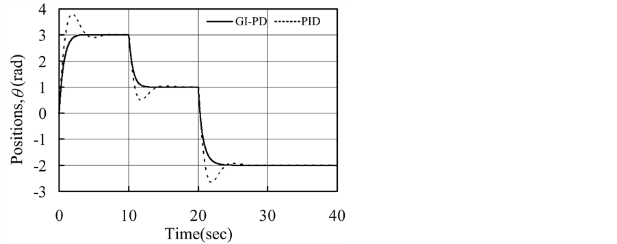
Figure 1. System output under the normal case.

Figure 2. System output under the perturbed cases.
7. Conclusion
In conjunction with a second order uncertain nonlinear system, this paper makes some comparisons between PID control and GI-PD control. The main contributions are: under GI-PD control, it is demonstrated that: 1) the system matrix can be stabilized more easily; 2) it is more effective to deal with the uncertain nonlinear actions; 3) the trouble caused by integrator windup is resolved in principle, and then it has the better control performance; 4) the harmonization of the integral control action and PD control action can be achieved. Moreover, design example and simulation results verify the justification of our conclusions again. All these means that GI-PD control has the stronger robustness and higher control performance than PID control. Consequently, GI-PD control has broader application prospects than PID control.
Cite this paper
BaishunLiu,BinHe,XiangqianLuo, (2015) On the Comparisons of PID and GI-PD Control. Engineering,07,387-394. doi: 10.4236/eng.2015.77035
References
- 1. Knospe, C.R. (2006) PID Control. IEEE Control Systems Magazine, 26, 30-31.
http://dx.doi.org/10.1109/MCS.2006.1580151 - 2. Liu, B.S. and Tian, B.L. (2009) General Integral Control. Proceedings of the International Conference on Advanced Computer Control, Singapore, 22-24 January 2009, 136-143.
http://dx.doi.org/10.1109/icacc.2009.30 - 3. Liu, B.S., Luo, X.Q. and Li, J.H. (2013) General Concave Integral Control. Intelligent Control and Automation, 4, 356-361.
http://dx.doi.org/10.4236/ica.2013.44042 - 4. Liu, B.S., Luo, X.Q. and Li, J.H. (2014) General Convex Integral Control. International Journal of Automation and Computing, 11, 565-570.
http://dx.doi.org/10.1007/s11633-014-0813-6 - 5. Liu, B.S. (2014) Constructive General Bounded Integral Control. Intelligent Control and Automation, 5, 146-155.
http://dx.doi.org/10.4236/ica.2014.53017 - 6. Liu, B.S. (2014) On the Generalization of Integrator and Integral Control Action. International Journal of Modern Nonlinear Theory and Application, 3, 44-52.
http://dx.doi.org/10.4236/ijmnta.2014.32007 - 7. Liu, B.S. and Tian, B.L. (2012) General Integral Control Design Based on Linear System Theory. Proceedings of the 3rd International Conference on Mechanic Automation and Control Engineering, 5, 3174-3177.
- 8. Liu, B.S. and Tian, B.L. (2012) General Integral Control Design Based on Sliding Mode Technique. Proceedings of the 3rd International Conference on Mechanic Automation and Control Engineering, 5, 3178-3181.
- 9. Liu, B.S., Li, J.H. and Luo, X.Q. (2014) General Integral Control Design via Feedback Linearization. Intelligent Control and Automation, 5, 19-23.
http://dx.doi.org/10.4236/ica.2014.51003 - 10. Liu, B.S., Luo, X.Q. and Li, J.H. (2014) General Integral Control Design via Singular Perturbation Technique. International Journal of Modern Nonlinear Theory and Application, 3, 173-181.
http://dx.doi.org/10.4236/ijmnta.2014.34019 - 11. Liu, B.S. (2015) Equal Ratio Gain Technique and Its Application in Linear General Integral Control. International Journal of Modern Nonlinear Theory and Application, 4, 21-36.
http://dx.doi.org/10.4236/ijmnta.2015.41003 - 12. Liu, B.S. (2015) Power Ratio Gain Technique and General Integral Control. Applied Mathematics, 6, 663-669.
http://dx.doi.org/10.4236/am.2015.64060 - 13. Khalil, H.K. (2007) Nonlinear Systems. 3rd Edition, Electronics Industry Publishing, Beijing, 551, 449-453.