Engineering
Vol. 2 No. 10 (2010) , Article ID: 3177 , 8 pages DOI:10.4236/eng.2010.210100
Geometric Inversion of Two-Dimensional Stokes Flows – Application to the Flow between Parallel Planes
Université Européenne de Bretagne, France
INSA, LGCGM, EA3913, F-35708 RENNES
E-mail: mustapha.hellou@insa-rennes.fr
Received May 17, 2010; revised July 21, 2010; accepted September 25, 2010
Keywords: Inversion Transformation, Geometric Inversion, Stokes Flow, Viscous Eddies, Flow around a Cylinder, Microflow
ABSTRACT
Geometric inversion is applied to two-dimensional Stokes flow in view to find new Stokes flow solutions. The principle of this method and the relations between the reference and inverse fluid velocity fields are presented. They are followed by applications to the flow between two parallel plates induced by a rotating or a translating cylinder. Thus hydrodynamic characteristics of flow around circular bodies obtained by inversion of the plates are thus deduced. Typically fluid flow patterns around two circular cylinders in contact placed in the centre of a rotating or a translating circular cylinder are illustrated.
1. Introduction
Geometric inversion is a type of transformation of the Euclidean plane. This transformation preserves angles and map generalized circles into generalized circles, where a generalized circle means either a circle or a line (a circle with infinite radius). One of the main properties of this method is the transformation of a straight line to a circle. Many difficult problems in geometry become much more tractable when an inversion is applied.
In engineering, the geometric inversion could be very useful to solve complex problems. For example, in fluid mechanics, the equation of two-dimensional Stokes flow remains valid in the new coordinates system obtained by inversion. Thus two-dimensional Stokes flow around certain bodies presenting circular shape appears less difficult to calculate by inversion of flow in channels of parallel walls than by direct calculation using polar coordinates. Although this method is rather general, we will apply it to the case of cellular flows (recirculation flow) presenting viscous eddies. In fact these flows are characterized by the presence of dividing streamlines (separating streamlines) which also give by inversion in the new geometry dividing streamlines.
Much attention has been paid to the steady viscous flow between parallel plates at low Reynolds number (Stokes flow) because of its theoretical importance and also its engineering applications. The particular case of the flow with vanishing velocity to zero when  (i.e. flow with mean rate equal zero) has been widely studied by authors motivated among others by separation phenomena. Thus, after the pioneering work of [1] who presented predictions of cellular motion in Stokes regime between parallel walls, theoretical works like those of [2] and [3] demonstrate the existence of such cellular flow. The corresponding authors showed that, independently of the motion source, any two-dimensional flow with mean rate null in a channel presented necessarily cellular motion composed by successive counter rotating eddies bounded by separating streamlines reattaching the walls. In order to examine the influence of the motion source, accurate computations for various motion sources have been performed [4-16]. Stokes flows and particularly cellular flows could be encountered in numerous applications in physics, biophysics, chemistry and MEMS (Micro and ElectroMechanical Systems) where microflows appear. The particularity of these applications is that they use microchannels [17-19]. Thus, several theoretical and numerical results are available. They could be useful to obtain by inversion transformation the structure and the features of Stokes flows around bodies of circular shape. This transformation is also useful to obtain flow around bodies with complex shape for which the direct calculation could be tiresome.
2. Geometric Inversion-Definitions and Properties
Inversion is the process of transforming points M to a corresponding set of points N known as their inverse points. Two points M and N drawn in Figure 1 are said to be inverses with respect to an inversion circle having inversion centre O and inversion radius R0 if N is the perpendicular foot of the altitude of the triangle OQM, where Q is a point on the circle such that OQ┴QM.
If M and N are inverse points, then the line L through M and perpendicular to OM is called a “polar” with respect to point N, known as the “inversion pole”. In addition, the curve to which a given curve is transformed under inversion is called its inverse curve (or more simply, its “inverse”).
From similar triangles, it immediately follows that the inverse points M and N obey to:
 or
or  (1)
(1)
where the quantity is known as the circle power or inversion power [20].
The general equation for the inverse of the point  relative to the inversion circle with inversion centre
  and inversion radius
  is given by
 ,
,  (2)
(2)
Note that a point on the circumference of the inversion circle is its own inverse point. In addition, any angle inverts to an opposite angle.
Treating lines as circles of infinite radius, all circles invert to circles. Furthermore, any two nonintersecting circles can be inverted into concentric circles by taking the inversion centre at one of the two so-called limiting points of the two circles [20], and any two circles can be inverted into themselves or into two equal circles. Or-

Figure 1. Geometric inversion – definition.
thogonal circles invert to orthogonal circles. The inversion circle itself, circles orthogonal to it, and lines through the inversion centre are invariant under inversion. Furthermore, inversion is a conformal map, so angles are preserved. Note that a point on the circumference of the inversion circle is its own inverse point. In addition, any angle inverts to an opposite angle.
The property that inversion transforms circles and lines to circles or lines (and that inversion is conformal) makes it an extremely important tool of plane analytic geometry. Figure 2 shows a simple example of application of geometric inversion.
The circle with dashed lines is the inversion circle of centre O and radius . Let take for example
 , the distance
  and the distance
 . Let’s make inversion of the straight lines L and L’ with centre O and power
 , we obtain the circles C and C’. The points N and Q are respectively the inverse images of the points M and P. The distances ON and OQ, calculated by using Equation (1), are
  and
and . Thus the radii of the circles C and C’ are respectively
  and
and .
.
In Figure 3 we present the classical example of inversion of a square relatively to a circle inscribed in this square. This inversion image becomes more complex if the number of squares is increased (see Mathematica Notebook presenting inversion of a grid).

Figure 2. Inversion of two parallel straight lines.

Figure 3. Inversion of a square. The inversion centre coincides with the square centre.
Figure 4 illustrates the inversion of parabola. This transformation leads to a cardiod defined in Figure 4(c). It’s worth to note that the change of the inversion centre leads to other figures of inversion.
3. Inversion Transformation of Stokes Flow
Let  be the stream function of a plane Stokes flow denoted F0 where
 . This flow is governed by the biharmonic equation:
 (3)
(3)
The function  is necessarily expressed by:
 (4)
(4)
(see[21]). Introducing the complex variable , it follows that the function
  can be written in a form similar to Equation (3). Consequently
  is likewise biharmonic and represents therefore the stream function of an other Stokes flow denoted thereafter F1.
Let  be a point of F0 and
  its homologous in the flow field F1 obtained by the positive inversion transformation of power a and centre O defined by Equation (1). It follows:
 (5)
(5)
And it’s easy to show that :
 (6)
(6)
The velocity components in polar coordinates framework of centre O on the homologous points are readily found to be:
 ;
; (7)
(7)
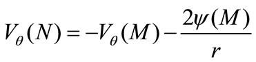
Hereafter, flow on which we apply the inversion method (Flow F0) is called reference flow. Now let F0 be a reference flow around a fixed body C0 and F1 is the equivalent flow in the proximity of the inverse fixed body C1. Assuming that the body C1 is at rest, by virtue of Equation (7), the non slip conditions on C1 are satisfied only for  on C0. However, we can add a constant which yields
  on this body without modifying F0. In this condition, an additional velocity is therefore added to F1 in order to ensure the non slip conditions on C1. Hence, the knowledge of the stream function field of F0 permits to determine the features of F1. Nevertheless, the inversion of a streamline of F0 does not give a streamline of F1 unless this streamline is a circle or of value
 . Thus in order to draw the streamlines, it would be necessary to calculate the stream function field of F1 by using Equation (6) and one can deduce straightforward the desired streamlines of F1. It is worth noting that the relations of equivalence between F0 and F1 for the other physical quantities (velocity, pressure, vorticity,…) can be determined without any particular problem.
4. Characteristics of the Cellular Flow between Parallel Plane Walls
The stream function of two dimensional Stokes flow with zero mean rate between parallel walls of a long rectangular channel has been found by [3], [5], [7] and [8] to be:
 (8)
(8)
where the functions Gn(y) have the following expressions according to the flow is antisymmetric

Figure 4. Inversion of a parabola (1996 © 2010 by Xah Lee). (a) inversion centre coincides with the focus of the parabola; (b) inversion centre coincides with the cusp of the parabola; (c) Cardioid can be defined as the trace of a point on a circle that rolls around a fixed circle of the same size without slipping.
 ( Equation (9)), respectively symmetric
  (Equation (10)):
 (9)
(9)
 (10)
(10)
The linear combination of these basic flows can compose the stream function of a more general flow. The coefficients are arbitrary complex coefficients to be determined by the boundary conditions and 2y0 represents the width of the channel. The parameters
  are the complex roots of the following equations coming from the non slip conditions on the channel walls.
 (antisymmetric flow) (11)
 (symmetric flow) (12)
The real coefficients and
and  have been accurately computed by Bourot & Moreau [5]; their sign is chosen here such as
  for
for .
.
Each term of the stream function of Equation (8) denoted  is null infinitely many times as
  whatever the motion source may be. There is an infinity of dividing streamlines of value
  = 0 which attach the parallel walls where the stream function is likewise zero and divide thus the flow on successive eddies. The equation of these dividing streamlines is given by:
 (13)
(13)
where Pn(y) and Qn(y) represent the real and imaginary parts of Gn(y).
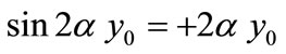
The Equation (13) means that the location of the dividing streamlines is periodic in the longitudinal direction. Hence, the axial length of each class n of eddies is constant and readily given by:
 (14)
(14)
Furthermore, angle at which the separating streamlines detach from the walls, i.e. the separation angle (angle T indicated in Figure 5), satisfies the equation:
 (15)
(15)
For n = 1, the separation angle is 58˚61 for an antisymmetric structure and 46˚25 for a symmetric one.
The ratio of the velocity on homologous points, i.e. points as S(x,y) and S’(x+Ln,y) (for example points S and S’indicated in Figure 5), is given by:
 (16)
(16)
For the same value of n, the velocity of the symmetric flow decays more than the velocity of the antisymmetric one. Thus, practically an arbitrary Stokes flow of zero mean rate between parallel plates becomes antisymmetric far from the motion source except when this source is strictly symmetric. Of course, numerical calculation of this arbitrary flow in the proximity of the motion source requires to conserve a sufficient number of terms  of the stream function, n = 20 or more ([5], [7] and [8]).
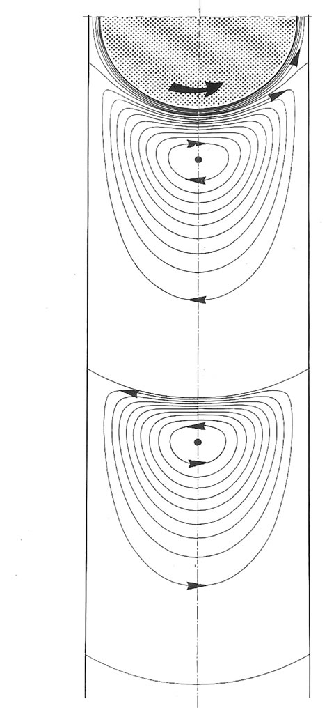
Figure 5 shows the streamlines of the theoretical flow corresponding to n = 1 for antisymmetric and symmetric conditions between parallel plates. The sequences of the dividing streamlines drawn in Figure 5 are located arbitrary since the motion source is not yet considered.
The stream function of the separating streamlines is zero hence they can be directly transformed. Thus associating to a point  of a separating streamline of F0 a point
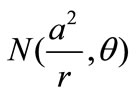 , we obtain a point of the corresponding separating streamline of the new flow F1. Consequently, the infinite cellular flow between parallel plates leads by inversion transformation to a finite cellular flow within the corners between the transformed bodies which the shape depends closely on the position of the inversion centre.
5. Applications
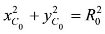
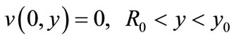
Antisymmetric and symmetric Stokes flows between parallel walls can be concretely realized by the uniform rotation respectively the uniform longitudinal translation of a cylinder midway between the parallel walls of a long rectangular channel filled with a viscous oil. The boundary conditions are the non slip conditions on the cylinder boundary and the matching conditions at x = 0 between the two semi-infinite domains. Precisely, these conditions are written as following:
0BAntisymmetric flow induced by a rotating cylinder
 with
with
 ,
,  ,
,
 ,
,
 (17)
(17)
where R0 represents the cylinder radius, V0 the cylinder velocity, u v the Cartesian components of the velocity and p the pressure (see Figure 6 for the notations).
Symmetric flow induced by a translating cylinder along the channel axis
 ,
, 
 (a)
(a) (b)
(b)
Figure 5. Theoretical flow between parallel walls [3]; (a) antisymmetric flow between parallel walls; (b) symmetric flow between parallel walls.
 ,
,
 (18)
(18)
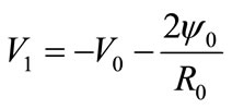
These flows, produced by rotating or translating cylinder, have been previously computed and examined by [22] and [8].
Now let apply the positive inversion to the domain bounded by parallel infinite walls. The centre of the cylinder is chosen as the inversion centre. The choice of the power a is not important. This parameter modify only the scale of the inverse field; let take a = y0 here. The transformation of the lines b0 and d0 representing the parallel walls leads to the tangent circles b1 and d1 (Figure 6). The rotating circle C0 of radius R0 gives a circle C1 of radius  which rotates with the velocity
 where
where  is the stream function on C0.

Figure 6. Delineation of the domain of reference composed by two parallel walls and a rotating circle of radius R0 (dashed lines ---) and the inverse domain composed by two circles in contact set in a rotating circle of radius R1 (solid lines — ). In this sketch, the power of the transformation is , thus
 .
.
In the case of translating cylinder on the axis or transversally to this axis with velocity  the stream function on C0 is
  respectively
 . By virtue of Equation (7), we see that the translation motion of a cylinder is invariant when applying the inversion transformation relatively to the centre. Consequently, we obtain by inversion a circle C1 moving with the same velocity. Note that inversion of a circle animated by both rotation and translation motions relatively to its centre leads likewise to a circle with the same motion.
Using results of the reference flows F0, published in [7] and [8], the purpose is now to obtain by the inversion method, the flow around two cylinders in contact set in a rotating or translating one. In the interest of brevity, we focused our attention to only the streamlines patterns.
The flow depicted in Figure 7(b) induced by a rotating cylinder around two fixed cylinders in contact is obtained by inversion of the flow presented in Figure 7(a). It exhibits an important cellular motion which is theoretically composed by an infinite sequence of closed viscous eddies, as demonstrated by [1] for a sharp corner. Their size diminishes as we approach the cusp whereas the size of eddies between parallel walls remains constant. The velocity decay is not constant but is important comparatively to the reference flow, about 4400 between the first and the second eddy and decreases to the limit of 358 in the neighbourhood of the contact line. Furthermore, the angles are invariant in the inversion transformation hence the angles subtended by the dividing streamlines are equivalent to those of the antisymmetric flow between parallel plates and found to be equal to 46˚ for the first line and 58˚61 for the next lines [2,3]. The first value of the contact angle is less than 58˚61 because it is influenced by the motion source.
 (a)
(a) (b)
(b)
Figure 7. (a) Streamline patterns of the flow between parallel plates induced by a rotating cylinder of radius ; (b) Streamline patterns of the flow around two cylinders in contact of radius
  centred inside an outer cylinder of radius
  (
( ) (structure obtained by inversion of structure a).
In the case of the translating cylinder, two configurations seem to be possible depending on whether the framework is absolute or relative. The inversion of the stream visualized by an observer attached to the absolute framework gives an instantaneous image of the flow around two cylinders in contact placed in the centre of the fluid domain bounded by a cylinder translating in the direction parallel to the contact plane, Figure 8(a). We see a symmetric cellular flow with an extent relatively small
 (a)
(a) (b)
(b) (c)
(c)
Figure 8. Streamlines around two cylinders in contact of radius  centred inside an outer cylinder of radius
  (
( ). The point of contact is located at the enclosure centre; (a) Two cylinders in contact fixed in a translating one; (b) Two cylinders in contact translating in the direction of the contact plane inside a fixed cylinder enclosure; (c) Two cylinders in contact rotating inside a fixed cylinder enclosure.
compared to the antisymmetric one. Note that adding the constant , leads to the more practical problem of two cylinders in contact translating in a fixed cylindrical enclosure whose the streamlines are presented in Figure 8(b). The relative reference flow regarded by an observer attached to the translating cylinder centre is equivalent to the flow around a fixed cylinder induced by translation of the walls. The inversion of this flow leads to the flow produced by two counter rotating cylinders in a fixed cylindrical enclosure, Figure 8(c). There is no separating streamlines because the corresponding reference stream is not of zero mean rate.
Figure 9(a) presents an example of a flow obtained by a rotating cylinder decentred from the axis of a channel of parallel plates with the distance d. If the inversion centre coincides with the cylinder centre, the inversion of the parallel walls leads to two cylinders in contact of different radius. The inversion of the flow leads to the flow drawn in Figure 9(b).
 (a)
(a)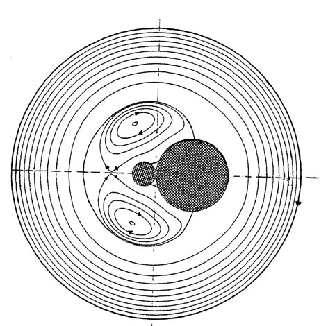 (b)
(b)
Figure 9. Inversion of the fluid flow between parallel walls due to a rotating cylinder of radius R1 = 0.25y0 decentred with the quantity d = 0.5y0 . Inversion of this flow; (a) Original flow; (b) Inversion of this flow.
6. Conclusions
For a two dimensional Stokes field corresponds theoretically by inversion an infinity of Stokes flows because the inversion centre can be any point of the  plane. For example, in the case of the flow between parallel plates, choosing this centre position on the
  axis normal to the parallel plates, provide solutions to flows around two unequal cylinders in contact internally or externally or around a cylinder in contact with a plane. Nevertheless, this centre would be suitably chosen otherwise the motion source obtained by inversion can be out of physical sense. For example, the inversion of the flow relatively to a point which is not the centre of a rotating cylinder leads to a flow across the inverse cylinder. Thus, useful configurations seem to be obtained essentially when the inversion centre coincides with the cylinder centre. From a general point of view, the inversion transformation is an interesting method which can be wide with various problems even apart from the fluid mechanics (electricity, chemistry, engineering processes, …) but a precaution in the choice of the position of the centre of inversion is necessary.
REFERENCES
- H. K. Moffatt, “Viscous and Resistive Eddies near a Sharp Corner,” Journal of Fluid Mechanics, Vol. 18, No. 1, 1964, pp. 1-18.
- M. E. O’ Neill, “On Angles of Separation in Stokes Flow,” Journal of Fluid Mechanics, No. 133, 1983, pp. 427-442.
- J. M. Bourot, “Sur la structure cellulaire des écoulements plans de Stokes, à debit moyen nul, en canal indéfini à parois parallèles,” Comptes rendus de l'Académie des sciences, Vol. 298, Serie II, 1984, pp. 161-164.
- C. Shen and J. M. Floryan, “Low Reynolds Number Flow over Cavities,” Physics of Fluids, Vol. 28, No. 11, 1985, pp. 3191-3202.
- J. M. Bourot and F. Moreau, “Sur l’utilisation de la série cellulaire pour le calcul d’écoulements plans de Stokes en canal indéfini: Application au cas d’un cylindre circulaire en translation,” Mechanics Research Communications, Vol. 14, No. 3, 1987, pp. 187-197.
- P. Carbonaro and E. B. Hansen, “Transient Stokes Flow in a Channel Driven by Moving Sleeves,” ASME Journal of Applied Mechanics, Vol. 57, No. 4, 1990, pp. 1061 -1065.
- M. Hellou and M. Coutanceau, “Cellular Stokes Flow Induced by Rotation of a Cylinder in a Closed Channel,” Journal of Fluid Mechanics, No. 236, 1992, pp. 557-577.
- F. Moreau and J. M. Bourot, “Ecoulements cellulaires de Stokes produits en canal plan illimité par la rotation de deux cylindres,” Journal of Applied Mathematics and Physics, Vol. 44, No. 5, 1993, pp. 777-798.
- P. N. Shankar and M. D. Deshpande, “Fluid Mechanics in the Driven Cavity,” Annual Review of Fluid Mechanics, No. 32, 2000, pp. 93-136.
- J. T. Jeong, “Slow Viscous Flow in a Partitioned Channel,” Physics of Fluids, Vol. 13, No. 6, 2001, pp. 1577 -1582.
- M. Hellou, “Structures d'écoulements de Stokes dans une jonction bidimensionnelle de canaux,” Mécanique & Industries, Vol. 4, No. 5, 2003, pp. 575-583.
- C. Y. Wang, “Slow Viscous Flow between Hexagonal Cylinders,” Transport in Porous Media, Vol. 47, No. 1, 2002, pp. 67-80.
- C. Y. Wang, “The Recirculating Flow due to a Moving Lid on a Cavity Containing a Darcy–Brinkman Medium,” Applied Mathematical Modelling, Vol. 33, No. 4, 2009, pp. 2054-2061.
- A. H. Abd El Naby and M. F. Abd El Hakeem, “The Flow Separation through Peristaltic Motion of PowerLaw Fluid in Uniform Tube,” Applied Mathematics Sciences, Vol. 1, No. 26, 2007, pp. 1249-1263.
- D. van der Woude, H. J. H. Clercx, G. J. F. van Heijst and V. V. Meleshko, “Stokes Flow in a Rectangular Cavity by Rotlet Forcing,” Physics of Fluids, Vol. 19, No. 8, 2007, pp. 083602-083602-19.
- M. Zabarankin, “Asymetric Three-diemensional Stokes Flows about Two Fused Equal Spheres,” Proceedings of the Royal Society A: Mathematical, Physical and Engineering Sciences, Vol. 463, No. 2085, 2007, pp. 2329 -2350.
- J. P. Brody, P. Yager, R. E. Goldstein and R. H. Austin, “Biotechnology at Low Reynolds Numbers,” Biophysical Journal, Vol. 71, No. 6, 1996, pp. 3430-3441.
- J. Yeom, D. D. Agonafer, J.-H. Han and M. A. Shannon, “Low Reynolds Number Flow across an Array of Cylindrical Microposts in a Microchannel and Figure-of-Merit Analysis of Micropost-Filled Microreactors,” Journal of Micromechanics Microengineering, Vol. 19, No. 6, 2009.
- C. Y. Wang, “Flow through a Finned Channel Filled with a Porous Medium,” Chemical Engineering Science, Vol. 65, No. 5, 2010, pp. 1826-1831.
- H. S. M. Coxeter, “Introduction to Geometry,” 2nd Edition, Wiley, New York, 1969, pp. 77-83.
- M. A. Laurentiev and B. V. Chabat, “Les méthodes de la théorie des fonctions de la variable complexe,” traduit du russe par Damadian H., Ed., Mir 1972, 1977.
- R. Bouard and M. Coutanceau, “Etude théorique et expérimentale de l’écoulement engendré par un cylindre en translation uniforme dans un fluide visqueux en régime de Stokes,” Journal of Applied Mathematics and Physics, Vol. 37, No. 5, 1986, pp. 673-684.